Tab Overview

For the description of the overview tab first the standard example of a business park and neighbouring ciy will be used. In the end of this page a small guide for filling out this tab from scratch will be given.

The overview tab for the standard example looks the following:

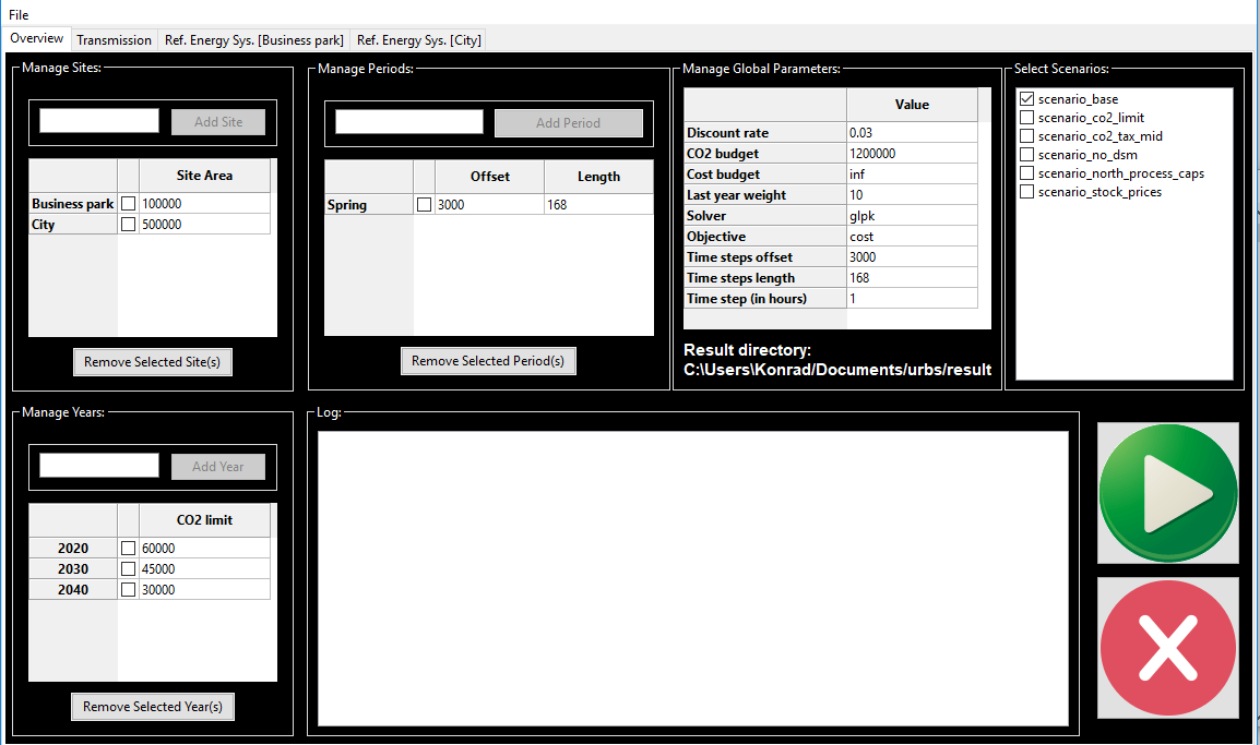
It is split into 6 main parts, all of which will be presented separately in the following.

Manage Sites

In the top left hand side the locations (sites) of the model are specified.

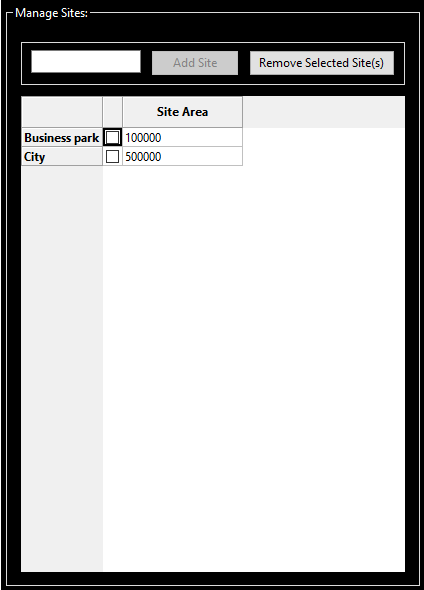
Each location has a designated area. For energy conversion units a capacity dependent area can bedefined and it is total available area that is restricted here per site. The area can be specified by clicking in the text field next to the checkbox and entering the desired number there (‘inf’ is also possible if no restriction is desired). You can add a new site by entering its name into the text line next to the Add Site button and clicking it. A site can be removed by first checking the checkbox next to the site name and then clicking the Remove Selected Site(s) button.

Manage Years

In the bottom left hand part of the overview tab you can manage the desired modeled years. These years are then the support years for the intertemporal modeling. It is also possible to enter just one year for a non-intertemporal, single year optimization.

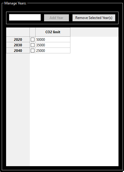
For each Year total allowed CO2 emissions can be specified. The energy system is then only allowed to emit the specified amount of CO2 across all modeled sites. The allowed annual emissions can be specified by clicking in the text field next to the checkbox and entering the desired number there (‘inf’ is also possible if no restriction is desired). You can add a new year by entering its name into the text line next to the Add Year button and clicking it. A modeled year can be removed by first checking the checkbox next to the year and then clicking the Remove Selected Year(s) button.

Manage Global Parameters

The upper middle part of the overview tab is used to specify global parameters.

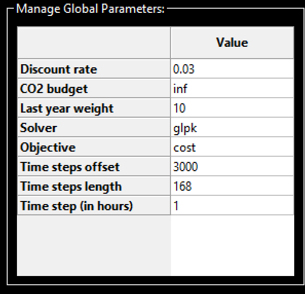
The global parameters are set by clicking on the field next to the quantity. In all cases except for Solver and Objective a number has to be entered. In the two cases singled out a drop down menu appears which offers the allowed choices. The parameters are:

• Discount rate: This value gives the discount rate that is used for intertemporal planning. It stands for the annual devaluation of money across the modeling horizon.
• CO2 budget: While the CO2 limit specified for each year limits the CO2 emissions across all sites within one modeled year, the CO2 budget sets a cap on the total emissions across all sites in the entire modeling horizon. If no restriction is desired enter ‘inf’ here. The CO2 budget is only active when the Objective is set to its default value ‘cost’.
• Cost budget: With this parameter a limit on the total system cost over the entire modeling horizon can be set. If no restriction is desired enter ‘inf’ here. The Cost budget is only active when the Objective is set to the value ‘CO2’.
• Last year weight: In intertemporal modeling each modeled year is repeated until the next modeled year is reached. This is done ba assigning a weight to the costs accrued in each of the modeled years. For the last modeled year the number of repetitions has to be set by the user here, where a high number leads to a stronger weighting of the last modeled year, i.e. of the final energy system configuration.
• Solver: Here you can specify the desired solver. When clicking on the field in column ‘Value’ a drop down menu opens where three solvers glpk, gurobi and cplex are listed as options. Note that only glpk is an open-source free ware for all users and included in the installation package. The other two solvers are commercial and have to be bought by the user separately.
• Objective: Here you can chose which quantity is to be minimized by the optimization process. There are currently two options ‘cost’ (default) and ‘CO2’. You can chose them in a drop down menu that occurs when you click into the ‘Value’ column.
• Time step offset/length: The next two global parameters specify which of the time steps given as parameters are to be considered by the model. The optimization will start at the value ‘offset+1’ and end at ‘offset+length’
• Time step (in hours): Many parameters are given to the model as time series. With this global parameter you can specify how long each entry of a time series is in hours.

Manage plot periods

To the right of the global parameters the plot periods can be defined. This is necessary since standard graphs become large and difficult to read if the optimization horizon is much longer than a week. The corresponding section on the screen looks like the following:

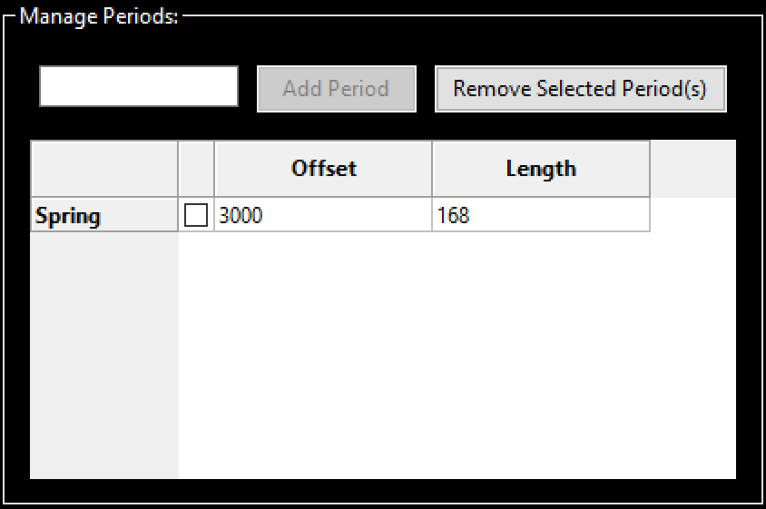
You can add new plot periods by specifying a name in the text field in the top section of the sub-window and then clicking the ‘Add Period’ button. The corresponding period will then appear in the lower section of the sub-window. You then have to specify the strating time step and the duration in the columns denoted ‘Offset’ and ‘Length’, respectively. For removing a plot period check the checkbox and then click the ‘Remove Selcted Period(s)’ button in the top section of the sub-window.

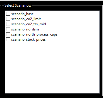
Scenarios

In the upper right hand section of the screen scenarios can be specified. These refer to variations in the input parameters which can be specified in functions in the subfolder ‘urbs’ in file ‘scenarios.py’. A few standard examples are listed already and can be chosen by checking the boxes next to their names.

Adding a new scenario is currently not a simple task and more for expert users. To do so you have to do 2 things.

1. Define a new scenario function in script ‘urbs/scenarios’
2. Make the function available for the GUI by adding it to the scenario list in the end of file ‘gui/Controller.py’.

Model running and supervision

The lower right hand part of the screen is dedicated to model running and supervision. With the ‘Play’ button a model run is started and can be interrupted with the red ‘Stop’ button. The lower section displays the log file of the model run.