Modeling nuggets

Here you can find a collection of non-trivial modeling ideas that can be used in linear energy system modeling with urbs. It is meant for more advanced users and you should fully understand the two standard examples mimo-example and Business park before proceeding. What follows is a loose collection of modeling approaches and does not follow any internal logic.

Different operational modes

For many power plants as, e.g., combined heat and power plants (CHP) there are different modes of operation. These and intermediate states between the extremes can be well captured in urbs models using the approach sketched in the following picture:

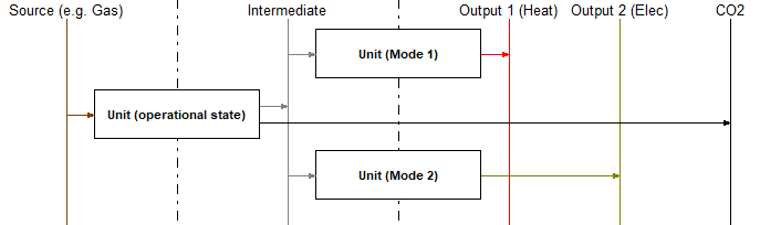
Here the vertical lines represent the commodities and the rectangle are processes. The arrows indicate in- and output commodities of the processes. In the case shown the power plant ‘Unit’ would be able to operate between a state where only ‘Output 1’ comes out and a state where only ‘Output 2’ comes out. The two extreme cases can, however, also be chosen as combinations of both outputs already.

The idea behind the figure is the following: The commodity ‘Intermediate’ is to be produced exclusively by the process ‘Unit (operational state)’. It thus simply tracks the throughput of this process. Due to the vertex rule (Kirchhoff´s current law) the commodity ‘Intermediate’ once produced needs to be consumed immediately. This can happen either via ‘Unit (Mode 1)’, ‘Unit (Mode 2)’ or a linear combination of both. The result is then the desired choice for the optimizer between states formed by linear combinations of the two modes. The commodity ‘Intermediate’ is best chosen as a Stock commodity where either the price is set to infinity or the maximum allowed usage per hour, or year (or both) is set to zero. This ensures that the commodity has to be produced by the process and cannot be bought from an external source, which for the present case would of course be absurd.

All process parameters and the setting of part load, time variable efficiency etc. is best done for the ‘Unit (operational state)’ process. The two other processes should in turn be used as mathematical entities that are defined by their ‘process commodity’ input only.

Proportional operation

Often many individual consumers are lumped together in one site. If a demand of these consumers is then met by a collection of decentral units it is important that the different technology options for these decentral units each fulfill a fixed fraction of the demand in each time step. This means that the different technology options are proportional to each other and the demand.

This behavior can be enforced by the following design:

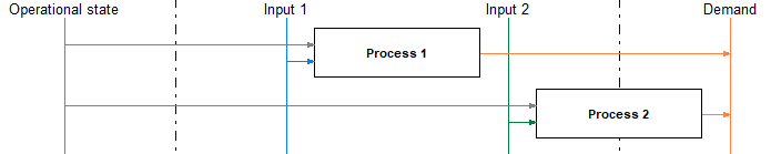
Here the vertical lines represent the commodities and the rectangle are processes. The arrows indicate in- and output commodities of the processes.

For the desired result the commodity ‘Operational state’ has to be of type SupIm and the corresponding time series has to be set as the normalized demand. in this way the optimizer can still size the two technology options ‘Process 1’ and ‘Process 2’ optimally while being forced to operate them proportionally to each other and to the demand. Other input or output (not shown) commodities can then be associated with the process operation as usual and will be dragged along by the forced operation.

Scenario generation

For a sensitivity analysis, it might be helpful to not manually create all scenario definitions automatically. For example, if one is interested in how installed capacities of PV and storage change the output, one might define ranges for each capacity. If there are four thresholds for the PV capacity and five for storage capacity, creating all 20 scenarios by hand is quite tiresome.

In this example, one wants to run an optimization with capacities 20 GW, 30 GW, 40 GW and 50 GW for PV and 50 GW, 60 GW, 70 GW, 80 GW and 90 GW for storage capacities.

Therefore, a function factory is created, which takes the values for PV and storage capacity and creates a scenario function out of it. This is done in the file scenarios.py:

def create_scenario_pv_sto(pv_val, sto_val):
    def scenario_pv_sto(data):
        # set PV capacity for all sites
        pro = data['process']
        solar = pro.index.get_level_values('Process') == 'Photovoltaics'
        pro.loc[solar, 'inst-cap'] = pv_val
        pro.loc[solar, 'cap-up'] = sto_val

        # set storage content capacity
        sto = data['storage']
        for site_sto_tuple in sto.index:
            sto.loc[site_sto_tuple, 'inst-cap-c'] = sto_val
            sto.loc[site_sto_tuple, 'cap-up-c'] = sto_val

        return data
    # define name for scenario dependent on pv and storage values
    scenario_pv_sto.__name__ = f"scenario_pv{int(pv_val/1000)}_sto{int(sto_val/1000)}"
    return scenario_pv_sto

In runme.py the following has to be added:

# define range for sensitvity
pv_vals = range(20000, 50001, 10000)
sto_vals = range(50000, 90001, 10000)

# create scenario functions
scenarios = []
for pv_val in pv_vals:
    for sto_val in sto_vals:
        scenarios.append(urbs.create_scenario_pv_sto(pv_val, sto_val))