Buy-Sell Documentation
This documentation explains the buy-sell-price feature of urbs. With it one can model time variant electricity prices from energy exchanges.
Introduction
The prices are independent of the amount of electricity purchased and fed in as
there is no feedback. The size of the modelled market has to be considered
small relative to the surrounding market.
To use this feature your excel input file needs an additional
Buy-Sell-Price sheet with the columns t containing the timesteps and
the columns Elec buy and Elec sell containing the buy and sell prices
by default in hourly € per MWh. In the Commodity sheet the price for
Elec at a Site has to be changed from a number to a string Buy or
Sell or a multiple of it for example 1,25xBuy.
For a more detailed description of the implementation have a look at the
Mathematical Documentation.
Exemplification
This section contains prototypical scenarios illustrating the system behaviour with time variant prices. Electricity can be moved locally with transmission losses and temporally with storage losses.
Fix Capacities - Fix Prices
All process, transmission and storage capacities and prices are predetermined and constant.
When is electricity purchased?
- if it is necessary that is the demand is greater than the total output capacity it is bought at every price
- if it is profitable that is if the buy price is lesser than the variable costs of the most expensive needed process
When is electricity fed-in?
- if it is possible and profitable that is if the demand is lesser than the total output capacity and the sell price greater than the cheapest currently not needed process
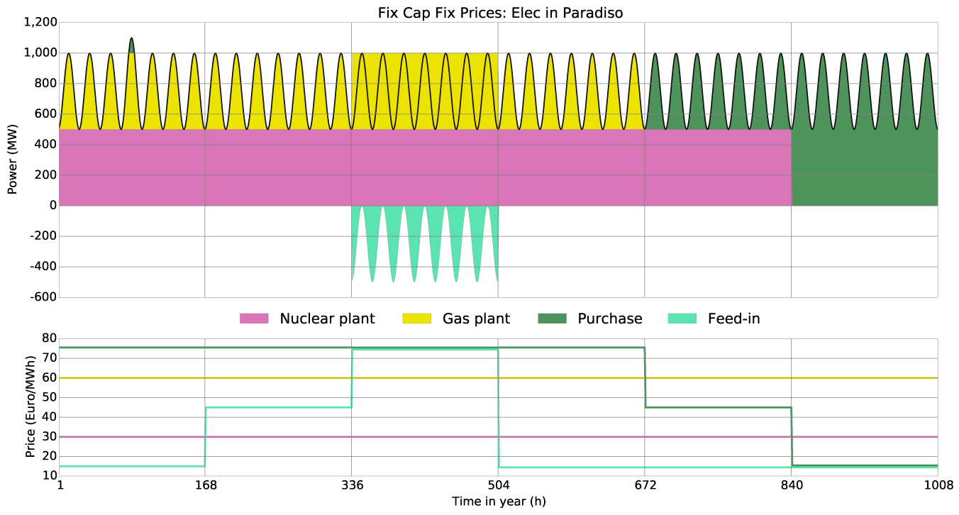
The following scenario illustrates the energy balance of the island Paradiso. It has a demand of 500-1000 MW that is supplied by a 1500 MW nuclear plant, a 1000 MW gas plant and a 1000 MW transmission cable, that connects the island grid with the continental grid. Both capacities and prices are fix.
| Process | eff | inst-cap | inst-cap-out | fuel-cost | var-cost | total-var-cost |
|---|---|---|---|---|---|---|
| Nuclear plant | 0.33 | 1500 | 500 | 5 | 5 | 10 |
| Gas plant | 0.50 | 1000 | 500 | 25 | 5 | 30 |
| Purchase | 1.00 | 1000 | 1000 | 15/45/75 | 0 | 15/45/75 |
| Feed-in | 1.00 | 1000 | 1000 | 15/45/75 | 0 | 15/45/75 |
The modelled timespan is 6 weeks with different fix prices each. In week 1 on the fourth day energy is purchased, because it is neccessary to cover the demand. In week 2 the sell price is higher than the variable costs of the nuclear plant, but lower than the variable costs of the cheapest not needed power plant: the gas plant. In week 3 the sell price excels even those costs making the production and selling of additional energy profitable. In week 4 buy prices are too high for purchase and sell prices to low for feed-in. In week 5 buy prices have dropped enough for purchased energy to replace energy produced by the gas plant. In week 6 they further dropped enough to even replace energy produced by the nuclear plant.
Fix Capacities - Variable Prices
All process, transmission and storage capacities are predetermined and constant, prices are varying over the modelled timespan.
When is electricity purchased?
- if it is necessary that is the demand is greater than the total output capacity it is bought at every price
- if it is profitable that is if the buy price is lesser than the current variable costs of the most expensive needed process or including storage costs lesser than future variable costs of the most expensive needed process
When is electricity fed-in?
- if it is possible and profitable that is if the demand is lesser than the total output capacity and the sell price greater than the cheapest currently not needed process
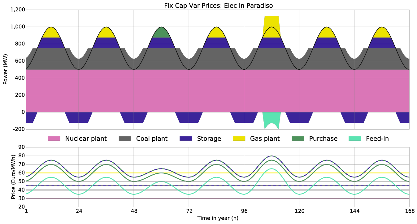
For the second scenario half of the gas plant is replaced by a coal plant. Additionally there is a new power limited energy storage with variable storage costs of 5 €/MWh. The load curve stays the same. Capacities are fix and prices are varying.
| Process | eff | inst-cap | inst-cap-out | fuel-cost | var-cost | total-var-cost |
|---|---|---|---|---|---|---|
| Nuclear plant | 0.33 | 1500 | 500 | 5 | 5 | 10 |
| Coal Plant | 0.40 | 625 | 250 | 11 | 5 | 16 |
| Gas plant | 0.50 | 500 | 250 | 25 | 5 | 30 |
| Storage | 1.00 | 125 | 125 | 2.5 | 5 | |
| Purchase | 1.00 | 1000 | 1000 | 50-75 | 0 | 50-75 |
| Feed-in | 1.00 | 1000 | 1000 | 35-65 | 0 | 35-65 |
The modelled timespan is 7 days. The buy price varies around the variable costs of the gas plant. But except for day 3 purchase is only a profitable substitute for energy from the gas plant at timesteps it is not needed. The sell price varies around the variable costs of the coal plant. But similar to the buy price except for day 5 it only allows production of energy for selling at timesteps it required to cover the demand instead. Producing and storing energy from the coal plant at timesteps with a low demand limited only by the storage power capacity is profitable, because it has total variable costs of 45 €/MWh and substitutes ebergy from the gas plant costing 60 €/MWh. At day 5 at noon the sell price exceeds the purchase price 12 hours before by 15 €/MWh. Even discounting storage costs of 5 €/MWh it would allow infinite arbitrage. But since the storage capacities are limited the opportunity costs of 15 €/MWh of substituting energy from the gas plant are higher than the 10 €/MWh profit margin it is not done.
Note
For trial e.g. of the result of greater storage capacities this
paradiso_2.xlsx
is the input file used for this scenario.
Variable Capacities - Variable Prices
All process, transmission and storage capacities are variable and determined at optimal total cost, prices are varying over the modelled timespan.
When is electricity purchased?
- if it is necessary that is the demand is greater than the total output capacity it is bought at every price
- if it is profitable that is if the buy price is lesser than the current variable costs of the most expensive needed process or including storage costs lesser than future variable costs of the most expensive needed process or it reduces the peak load allowing the capacity investments to be reduced in a way that overcompensates the additional costs in summary
When is electricity fed-in?
- if it is possible and profitable that is if the demand is lesser than the total output capacity and the sell price greater than the cheapest currently not needed process and does not prevent a total costs decrease by reduction of the capacity investments
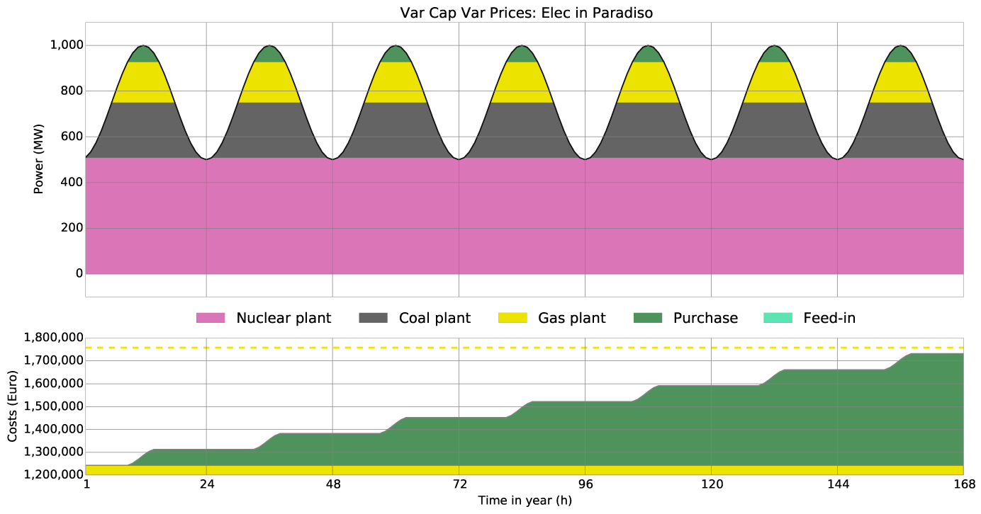
The next scenario is very similar to the previous one, only that this time all
capacities are initially 0 and investment in new capacities is done in a cost
optimal way. The ascencing order of variable prices is still nuclear plant -
coal plant - gas plan. The ascending order of fix costs, the sum of annual fix
costs fix-cost and annualized depreciations calculated from the investment
costs inv-cost, weighted average cost of capital wacc and economic life
time depreciation is the opposite: gas plant - coal plant - nuclear plant.
| Process | eff | inst-cap | inst-cap-out | fuel-cost | var-cost | total-var-cost |
|---|---|---|---|---|---|---|
| Nuclear plant | 0.33 | 0 | 0 | 5 | 5 | 10 |
| Coal Plant | 0.40 | 0 | 0 | 11 | 5 | 16 |
| Gas plant | 0.50 | 0 | 0 | 25 | 5 | 30 |
| Storage | 1.00 | 0 | 0 | 2.5 | 5 | |
| Purchase | 1.00 | 0 | 0 | 150-250 | 0 | 150-250 |
| Feed-in | 1.00 | 0 | 0 | 30-50 | 0 | 30-50 |
This scenario should demonstrate a typical composition of power plants. This is the result of each power plant being cost optimal for a certain range of full load hours per year leading nuclear energy to cover the base load and gas energy to cover the peak load. It should also demonstrate, why the purchase of energy that at the moment exceeds variable costs of power plants can be economically worthwhile as it reduces peak loads and decreases overall costs.
| Process | fix-cost | inv-costs | wacc | depreciation | anf | annuity | total-fix-cost |
|---|---|---|---|---|---|---|---|
| Gas plant | 2000 | 2250000 | 0.07 | 30 | 0.08 | 181319 | 183319 |
| Purchase | 0 | 0 | 0.07 | 0 | 0 |
The variable peak costs of purchased energy of 250 €/MWh clearly exceed the variable costs of the gas plant of 60 €/MWh. However the necessary transmission cables for purchasing energy are already needed anyways and do not require additional fix costs in this scenario while the gas plant has total annual fix costs of 183.319 €/MW throughput power and 362.639 €/MW output power. Focussing on one week reducing the needed output capacity by 1MW would save 6.955 €. As showed by the following diagramms this justifies the additional costs of 250 € - 60 € = 190 € per purchased MWh to an amount that reduces the peak load by 73 MW.
Note
For trial e.g. of the result of different storage capacities this
paradiso_3.xlsx
is the input file used for this scenario.
System support by variable prices
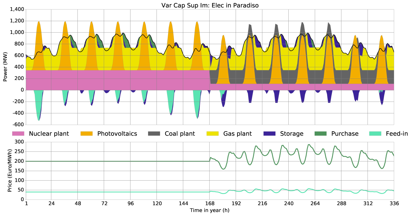
Making the prices a function proportional to demand and inversely proportional to intermittent supply is both a good approximation and can demonstrate the system support of such prices. Especially in case of photovoltaics it limits the installed capacity to a reasonable amount and/or encourages investment in storages. This leads to lower peak loads decreasing stress on the grid and a smoother residual demand increasing stability and autarky. Without variable prices storages will run a greedy operation strategy instead of peak shaving and put even more stress on the grid with large power gradients.
| Process | eff | inst-cap | inst-cap-out | fuel-cost | var-cost | total-var-cost |
|---|---|---|---|---|---|---|
| Nuclear plant | 0.33 | 0 | 0 | 5 | 5 | 10 |
| Coal Plant | 0.40 | 0 | 0 | 11 | 5 | 16 |
| Gas plant | 0.50 | 0 | 0 | 25 | 5 | 30 |
| Photovoltaics | 1.00 | 0 | 0 | 0 | 0 | 0 |
| Storage | 1.00 | 0 | 0 | 0 | 2.5 | 5 |
| Purchase | 1.00 | 0 | 0 | 150-250 | 0 | ~200 |
| Feed-in | 1.00 | 0 | 0 | 30-50 | 0 | ~40 |
The price function for the scenario was chosen as:
Buy price = 100 + 100 * Demand / mean(Demand) * (1.5 - SupIm)

Sell price = Buy Price / 5
The result is both more realistic and protective of the grid.
Arbitrage
Arbitrage is the profitable buying and selling of commodities exploiting price differences. For urbs this can be at one timestep or with storages between two different timesteps. It can lead the model to be unbounded, if the buy price at one time step is lower than the sell price or if the price difference between two different timesteps is large enough to finance storage investments. A simple solution to avoid that possibility is to add a large finite upper limit for storage capacities.