Workflow¶

This page is a step-by-step explanation on how to get one’s own model running. For the sake of an example, assume you want to investigate whether the (imaginary) state New Sealand with its four islands Vled Haven, Qlyph Archipelago, Stryworf Key, and Jepid Island would benefit by linking their islands’ power systems by costly underground cables to better integrate fluctuating wind power generation.

Prerequisites¶

You have followed the sections installation instructions and get started in the README, i.e. you can successfully execute an optimisation run with the example dataset mimo-example.xlsx with the example run script runme.py. These two files will serve as a scaffold for your own investigation.

Create a private development branch¶

Using git, create and directly checkout a new branch with a topical name. Good names should tell you the goal of a branch, so something along the lines of test1234 is no good name. For this project, newsealand looks like a good name:

$ git checkout -b newsealand

The private branch can be used to commit your own changes, while benefitting from new features/bug fixes that are pushed to the master branch on GitHub. Whenever you want to retreive those new changes, execute the following commands:

$ git fetch origin
$ git rebase origin/master

A full explanation of how to use git is beyond the scope of this documentation, so please refer to the Git book, especially chapter 1, 2, 3.

Create an input data file¶

Create a copy of the file mimo-example.xlsx and give it short, descriptive name newsealand.xlsx. Open it.

Go through the sheets, either adding, deleting or modifying rows. Keep the column titles as they are, because they are required by the model. Each title has a tooltip that explains the use of the parameter.

If you have created a development branch, this is a good time to add this file to version control:

$ git add newsealand.xlsx
$ git commit -m "added newsealand.xlsx"

Site, DSM and Buy-Sell-price¶

Note at the outset, that you do not have to worry about the three mentioned worksheets, since they are not used for this tutorial. You need to keep them, however, and modify them in order to avoid problems. First, specify the four desired Sites in Site and set all values to either NV() or inf. In the sheet DSM enter the four islands of New Sealand as sites into the corresponding fields and set all values in the columns cap-max-do and cap-max-up to 0. You do not need to change anything in sheet Buy-Sell-Price.

Commodity¶

Remove the rows with unneeded commodities, here everything except Gas, Elec, Wind, CO2, and Slack. New Sealand only uses these for power generation. While Slack is not needed, it makes debugging unexpected model behaviour much easier. Better keep it. Rename the sites to match the island names. The file should now contain 20 rows, 5 for each island.

Let’s assume that Jepid Island does not have access to Gas, so change the parameter max and maxperstep to 0. Island Stryworf Key does have a gas connection, but the pipeline can only deliver 50 MW worth of Gas power.

These steps result in the following table. The bolded values result from the assumptions described in the previous paragraphs. The other values are left unchanged from the example dataset:

Sheet **Commodity**; empty cells correspond to `=NV()` (*no value*) fields¶
Site	Commodity	Type	price	max	maxperstep
Jepid Island	CO2	Env		inf	inf
Jepid Island	Elec	Demand
Jepid Island	Gas	Stock	27.0	0.0	0.0
Jepid Island	Slack	Stock	999.0	inf	inf
Jepid Island	Wind	SupIm
Qlyph Archipelago	CO2	Env		inf	inf
Qlyph Archipelago	Elec	Demand
Qlyph Archipelago	Gas	Stock	27.0	inf	inf
Qlyph Archipelago	Slack	Stock	999.0	inf	inf
Qlyph Archipelago	Wind	SupIm
Stryworf Key	CO2	Env		inf	inf
Stryworf Key	Elec	Demand
Stryworf Key	Gas	Stock	27.0	inf	50.0
Stryworf Key	Slack	Stock	999.0	inf	inf
Stryworf Key	Wind	SupIm
Vled Haven	CO2	Env		inf	inf
Vled Haven	Elec	Demand
Vled Haven	Gas	Stock	27.0	inf	inf
Vled Haven	Slack	Stock	999.0	inf	inf
Vled Haven	Wind	SupIm

You have done some work already. It’s time for another commit. Instead of adding every changed file manually, you can add option -a to the commit, which adds all unstaged changes from git status to the next commit. With that:

$ git commit -am "changed commodities to 4 islands in newsealand.xlsx"

Note

From now on, commit yourself whenever you reach a point you want to be able to go back to later.

Process¶

First, remove any process from sheet Process-Commodity that consumes or produces a commodity that is no longer mentioned in sheet Commodity. For New Sealand, this leaves us with three processes: Gas plant, Slack powerplant, Wind park. The output ratio 0.6 of the Gas plant is the electric efficiency.

Sheet **Process-Commodity**¶
Process	Commodity	Direction	ratio
Gas plant	CO2	Out	0.2
Gas plant	Elec	Out	0.6
Gas plant	Gas	In	1.0
Slack powerplant	CO2	Out	0.0
Slack powerplant	Elec	Out	1.0
Slack powerplant	Slack	In	1.0
Wind park	Elec	Out	1.0
Wind park	Wind	In	1.0

With only these processes remaining, the sheet Process, needs some work, too. create an entry for each process that can be built at a given site. The upper capacity limits cap-up for each process are the most important figure. Qlyph Archipelago is known for its large areas suitable for wind parks up to 200 MW, only surpased by the great offshore sites of Jepid Island with 250 MW potential capacity. The other islands only have space for up to 120 MW or 80 MW. Gas plants can be built up to 100 MW on every island, except for Vled Haven, which can house up to 80 MW only.

Slack powerplants are set to an installed capacity inst-cap higher than the peak demand in each site, so that any residual load could always be covered. To make its use unattractive, you set the variable costs var-cost to 9 M€/MWh. This yields the following table:

Sheet **Process**¶
Site	Process	inst-cap	cap-lo	cap-up	max-grad	inv-cost	fix-cost	var-cost	wacc	depr.
Jepid Island	Gas plant	25	0	100	5	450000	6000	1.62	0.07	30
Jepid Island	Slack powerplant	999	999	999	inf	0	0	9000000.0	0.07	1
Jepid Island	Wind park	0	0	250	inf	900000	30000	0.0	0.07	25
Qlyph Archipelago	Gas plant	0	0	100	5	450000	6000	1.62	0.07	30
Qlyph Archipelago	Slack powerplant	999	999	999	inf	0	0	9000000.0	0.07	1
Qlyph Archipelago	Wind park	0	0	200	inf	900000	30000	0.0	0.07	25
Stryworf Key	Gas plant	25	0	100	5	450000	6000	1.62	0.07	30
Stryworf Key	Slack powerplant	999	999	999	inf	0	0	9000000.0	0.07	1
Stryworf Key	Wind park	0	0	120	inf	900000	30000	0.0	0.07	25
Vled Haven	Gas plant	0	0	80	5	450000	6000	1.62	0.07	30
Vled Haven	Slack powerplant	999	999	999	inf	0	0	9000000.0	0.07	1
Vled Haven	Wind park	0	0	80	inf	900000	30000	0.0	0.07	25

Transmission¶

On transmission, map the network topology of New Sealand. Vled Haven is the central hub of the state, with the other islands connected like a star shape. The investment costs are scaled according to the air distance from the population centers of each island. So Jepid Island with 1.1 M€/MW investment costs is more than twice as far away from Vled Haven than Ylyph Archipelago with only 0.5 M€/MW. Stryworf Key is somewhere between with 0.8 M€/MW. All investment costs are per direction. So the bidirectional cable costs are actually the summed inv-cost for both directions.

Sheet **Transmission**¶
Site In	Site Out	Transmission	Commodity	eff	inv-cost	fix-cost	cap-up	wacc	depr.
Jepid Island	Vled Haven	undersea	Elec	0.85	1100000	30000	inf	0.07	30
Qlyph Archipelago	Vled Haven	undersea	Elec	0.95	500000	15000	inf	0.07	30
Stryworf Key	Vled Haven	undersea	Elec	0.9	800000	22500	inf	0.07	30
Vled Haven	Jepid Island	undersea	Elec	0.85	1100000	30000	inf	0.07	30
Vled Haven	Qlyph Archipelago	undersea	Elec	0.95	500000	15000	inf	0.07	30
Vled Haven	Stryworf Key	undersea	Elec	0.9	800000	22500	inf	0.07	30

Storage¶

Storing electricity is possible only on Qlyph Archipelago, using an unsepcified technology simply labeled gravity here. To allow for parameterising a host of technologies, costs for both storage power and capacity can be specified independently. For most technologies, one of the costs will be dominating, so the other value can be set simply (near) zero to reflect that. The last parameter init specifies a) how full the storage is at the first time step and b) at least how full it must be at the final time step. That way, a short simulation duration may not just exhaust the storage.

Sheet **Storage** (1/2)¶
Site	Storage	Commodity	inst-cap-c	cap-lo-c	cap-up-c	inst-cap-p	cap-lo-p	cap-up-p	eff-in	eff-out
Qlyph Archipelago	gravity	Elec	0	0	inf	0	0	inf	0.95	0.95

Sheet **Storage** (2/2)¶
Site	Storage	Commodity	inv-cost-p	inv-cost-c	fix-cost-p	fix-cost-c	var-cost-p	var-cost-c	depr.	wacc	init
Qlyph Archipelago	gravity	Elec	500000	5	0	0.25	0.02	0	50	0.07	0.05

Hacks¶

In the base scenario, no limit on CO2 emissions from Gas plants is needed. Therefore, you set the value to inf:

Sheet **Hacks**¶
Name	Value
Global CO2 limit	inf

Time series¶

The only commodity of type SupIm is Wind, which you defined in sheet Commodity on all four islands. Therefore, in total 4 time series must be provided here, even if they are all zeros. As your data provider has not kept his promise to send you the data on time, you (ab)use the mimo-example.xlsx data once more, and simply use its time series. To get qualitatively correct results, you assign the best (3600 full load hours) to Jepid island, the second best to Vled Haven (3000 full load hours) and two copies of the worst time series (2700 full load hours) to Qlyph Archipelago and Stryworf Key. With that, you get the following table of capacity factors:

Sheet **SupIm**¶
t	Jepid Island.Wind	Qlyph Archipelago.Wind	Stryworf Key.Wind	Vled Haven.Wind
0	0.0	0.0	0.0	0.0
1	0.603	0.935	0.935	0.458
2	0.585	0.942	0.942	0.453
3	0.571	0.956	0.956	0.453
4	0.561	0.956	0.956	0.461
…	…	…	…	…

You make sure that both the island names and the commodity name exactly match the identifiers used on the other sheets.

For the demand, you also have no real data for now. But with some scaling (divide by 1000), the example series make for a good temporary demand time series. Vled Haven has the highest peak load with 75 MW, followed by Stryworf Key with 19 MW and the other islands with 8.2 MW each:

Sheet **Demand**¶
t	Jepid Island.Elec	Qlyph Archipelago.Elec	Stryworf Key.Elec	Vled Haven.Elec
0	0	0	0	0
1	4	4	11	43
2	4	4	10	41
3	4	4	10	40
4	4	4	10	40
…	…	…	…	…

Note

For reference, this is how newsealand.xlsx looks for me having performed the above steps.

Test-drive the input¶

Now that newsealand.xlsx is ready to go, start ipython in the console. Execute the following lines, best by manually typing them in one by one. (Hint: use tab completion to avoid typing out function or file names!)

First, load the data:

>>> import urbs
>>> input_file = 'newsealand.xlsx'
>>> data = urbs.read_excel(input_file)

data now is a standard Python dict. So data.keys() yields the worksheet names, while data['commodity'] contains the Commodity worksheet as a DataFrame. Now create a range:

>>> offset, duration = (3500, 14*24)
>>> timesteps = range(offset, offset + duration + 1)

[3500, 3501, ..., 3836]

Now you can create the optimisation model, then convert it to an optimisation problem that can be handed to the solver:

>>> prob = urbs.create_model(data, timesteps)

Now the only thing missing is the solver. It can be used through another object that is generated by the SolverFactory function from the pyomo package:

>>> import pyomo.environ
>>> from pyomo.opt.base import SolverFactory
>>> optim = SolverFactory('glpk')

Ignore the deprecation warning [1] for now. The solver object has a solve method, which takes the problem as an argument and returns a solution. For bigger problems, the next step can take several hours or even days. Therefore, you enable visible progress output by setting the option tee [2]. Additionally, you can save the output to a logfile using the logfile option:

>>> result = optim.solve(prob, logfile='solver.log', tee=True)

This results in roughly the following output appearing on the console:

GLPSOL: GLPK LP/MIP Solver, v4.55
[...]
GLPK Simplex Optimizer, v4.55
26275 rows, 22558 columns, 63630 non-zeros
Preprocessing...
14793 rows, 13120 columns, 35970 non-zeros
Scaling...
 A: min|aij| = 2.305e-003  max|aij| = 1.053e+000  ratio = 4.567e+002
GM: min|aij| = 3.606e-001  max|aij| = 2.773e+000  ratio = 7.691e+000
EQ: min|aij| = 1.300e-001  max|aij| = 1.000e+000  ratio = 7.691e+000
Constructing initial basis...
Size of triangular part is 14790
      0: obj =  3.000000000e+005  infeas = 2.158e+004 (3)
    500: obj =  2.443067336e+007  infeas = 8.024e+003 (3)
   1000: obj =  3.635166806e+011  infeas = 5.311e+003 (3)
*  1379: obj =  1.688377193e+012  infeas = 0.000e+000 (3)
[...]
*  5500: obj =  3.438413434e+007  infeas = 6.221e-014 (3)
*  5822: obj =  3.419699391e+007  infeas = 7.889e-031 (3)
OPTIMAL LP SOLUTION FOUND
Time used:   3.5 secs
Memory used: 25.3 Mb (26496968 bytes)
Writing basic solution to '<temporary.glpk.raw>'...
48835 lines were written

Finally, you can load the result back into the optimisation problem oject prob:

>>> prob.solutions.load_from(result)
True

This object now contains all input data, the equations and result data. If you store this object as a file, you can later always create new analyses from it. That’s what save() is made for:

>>> urbs.save(prob, 'newsealand-base.pgz')

This becomes especially helpful for large problems that take hours to solve. Back to the prob. To get a quick numerical overview on the most important result numbers, use report():

>>> urbs.report(prob, 'report.xlsx',prob.com_demand,prob.sit)

By default, this report only includes total costs and capacities of process, transmission and storage. By adding the optional third and fourth parameter, you can retreive timeseries listings of energy production per site. For now, you are only interested in electricity in Vled Haven:

>>> urbs.report(prob, 'report-vled-haven.xlsx',
...             ['Elec'], ['Vled Haven'])

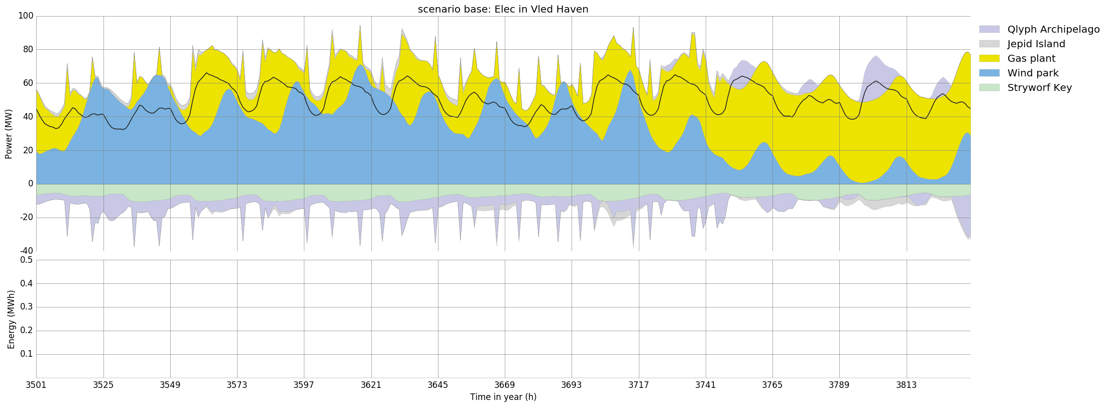
Then you finally want to see how the electricity production looks like. For that you use plot():

>>> %matplotlib
>>> fig = urbs.plot(prob, 'Elec', 'Vled Haven')

_images/newsealand_base-Elec-Vled-Haven.png

Depending on the plotting backend, you now either see a window with the plot (‘TkAgg’, ‘QtAgg’), or nothing. Either way, you can save the figure to a file using:

>>>  fig.savefig('newsealand-base-elec-vled-haven.png',
...              dpi=300, bbox_inches='tight')

The file extension determines how the output is written. Among the supported formats are jpg, pdf, png, svg and tif. Use png if raster images are needed and rely on pdf or svg for vector output. The dpi option is only used for raster images. bbox_inches='tight' removes unnecessary whitespace around the plot, making it suitable for inclusion in reports or presentations.

Create a run script¶

As it is quite tedious to perform the above actions by hand all the time, a script can automate these. This is where a runme.py script becomes handy.

Create a copy of the script file runme.py and give it a suitable name, e.g. runns.py.

Modify the scenario_co2_limit function. As the base scenario now has no limit, reducing it by 95 % does not make it finite. Therefore you set a fixed hard (annual) limit of 40 million tonnes of CO2 equivalent:

 def scenario_co2_limit(data):
     # change global CO2 limit
     hacks = data['hacks']
     hacks.loc['Global CO2 limit', 'Value'] = 40000
     return data

Next, set adjust the plot_tuples and report_tuples by replacing North, Mid and South by the four islands of Newsealand. Furthermore, you want to show imported/exported electricity in the plots in custom colors. So you modify the my_colors dict like this:

my_colors = {
    'Vled Haven': (230, 200, 200),
    'Stryworf Key': (200, 230, 200),
    'Qlyph Archipelago': (200, 200, 230),
    'Jepid Island': (215,215,215)}

Finally, you head down to the if __name__ == '__main__' section that is executed when the script is called. There, you change the input_file to your spreadsheet newsealand.xlsx and increase the optimisation duration to 14 days (14*24 time steps). For now, you don’t need the other scenarios, so you exclude them from the scenarios list:

 if __name__ == '__main__':
     input_file = 'newsealand.xlsx'
     result_name = os.path.splitext(input_file)[0]  # cut away file extension
     result_dir = prepare_result_directory(result_name)  # name + time stamp

     (offset, length) = (3500, 14*24)  # time step selection
     timesteps = range(offset, offset+length+1)

     # select scenarios to be run
     scenarios = [
         scenario_base,
         scenario_co2_limit]

     for scenario in scenarios:
         prob = run_scenario(input_file, timesteps, scenario, result_dir)

Note

For reference, here is how runns.py looks for me.

[1]	If you used Coopr 4.0, simply `import coopr.environ` before importing `SolverFactory`.

[2]	like the GNU tee output redirection tool.