Asynchronous ADMM implementation

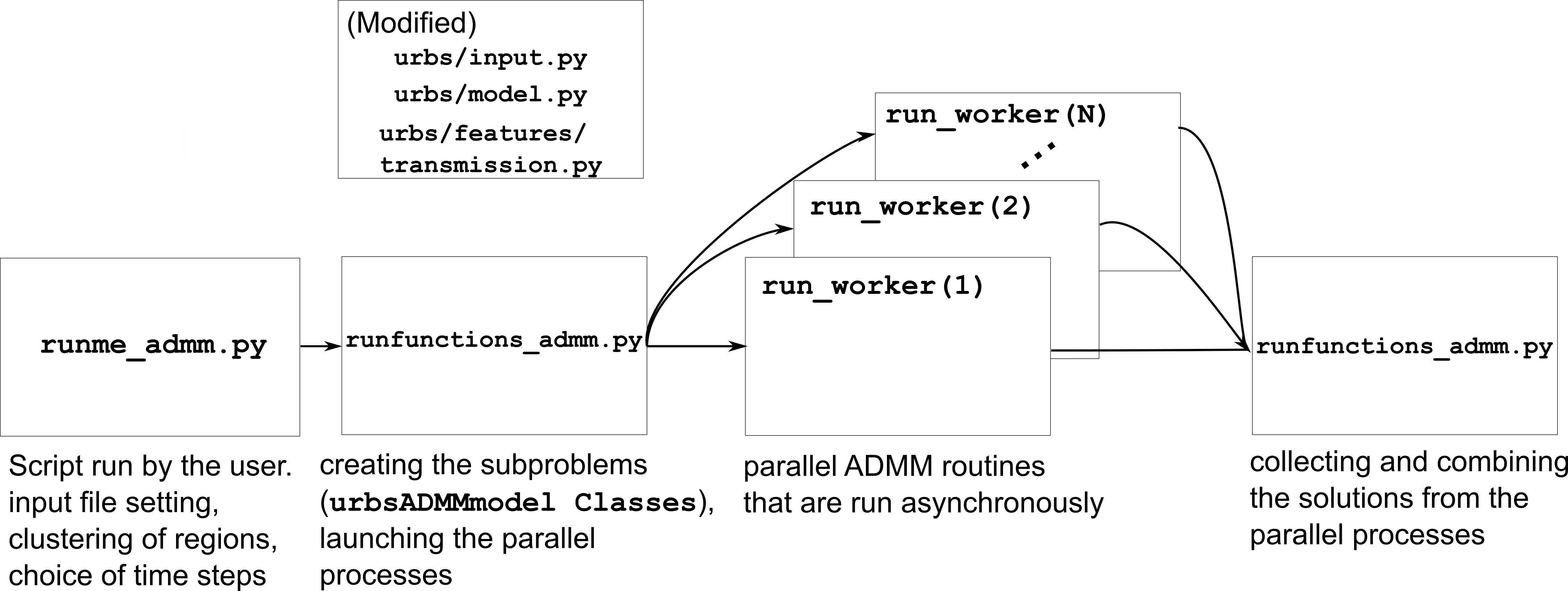
This section explains the implementation of the asynchronous ADMM module. The workflow of the asynchronous ADMM module is established in the following way:

runme_admm.py: runme_admm.py is the script that has to be run by the user, where the input file for the model, modelled time period and the cluster definition is made.

runfunctions_admm.py: runfunctions_admm.py is the script that is called by the runme_admm.py script. Here, the data structures for the subproblems is created, the submodels are built, and asynchronous ADMM processes are launched.

run_Worker.py: ADMM_async/run_Worker.py includes the function run_worker(), which is the parallel ADMM routine that are followed asynchronously by the parallel workers. The major argument of this function is a urbsADMMmodel class, whose methods are defined in the ADMM_async/urbs_admm_model.py script.

Moreover, minor additions/modifications were done on the following, already existing scripts:

• urbs/input.py
• urbs/model.py
• urbs/features/transmission.py

which will also be mentioned here.

The workflow of the ADMM implementation is illustrated as follows:

In the following, a walkthrough on the scripts involved will be given to establish understanding regarding how the ADMM implementation works.

runme_admm.py

Let us start with the imported packages:

import os
import shutil
import urbs
from urbs.runfunctions_admm import *
from multiprocessing import freeze_support

Besides the usual urbs imports os, shutil and urbs, the urbs.runfunctions module is imported as it contains the urbs.run_regional function that commences the ADMM routine. Moreover, to allow for parallel operation on Windows systems, the freeze_support function has to be imported from the multiprocessing package.

Moving on to the input settings:

The script starts with the specification of the input file, which is to be located in the same folder as script runme_admm.py:

# Choose input file
input_files = 'germany.xlsx'  # for single year file name, for intertemporal folder name
input_dir = 'Input'
input_path = os.path.join(input_dir, input_files)

Then the result name and the result directory is set:

result_name = 'Run'
result_dir = urbs.prepare_result_directory(result_name)  # name + time stamp

Input file is added in the result directory:

# copy input file to result directory
try:
    shutil.copytree(input_path, os.path.join(result_dir, input_dir))
except NotADirectoryError:
    shutil.copyfile(input_path, os.path.join(result_dir, input_files))
# copy run file to result directory
shutil.copy(__file__, result_dir)

The objective function to be minimized by the model is then determined (options: ‘cost’ or ‘CO2’):

# objective function
objective = 'cost'  # set either 'cost' or 'CO2' as objective

Then the specification of time step length and modeled time horizon is made:

# simulation timesteps
(offset, length) = (0, 8760)  # time step selection
timesteps = range(offset, offset+length+1)
dt = 1  # length of each time step (unit: hours)

Variable timesteps is the list of time steps to be modelled. Its members must be a subset of the labels used in input_file’s sheets “Demand” and “SupIm”. It is one of the function arguments to create_model() and accessible directly, so that one can quickly reduce the problem size by reducing the simulation length, i.e. the number of time steps to be optimised. Finally, the variable dt gives the width of each timestep, input in hours.

range() is used to create a list of consecutive integers. The argument +1 is needed, because range(a,b) only includes integers from a to b-1:

>>> range(1,11)
[1, 2, 3, 4, 5, 6, 7, 8, 9, 10]

An essential input for the ADMM module is the clustering scheme of the model regions:

clusters = [[('Schleswig-Holstein')],[('Hamburg')],[('Mecklenburg-Vorpommern')],[('Offshore')],[('Lower Saxony')],[('Bremen')],[('Saxony-Anhalt')],[('Brandenburg')],[('Berlin')],[('North Rhine-Westphalia')],
            [('Baden-Württemberg')],[('Hesse')],[('Bavaria')],[('Rhineland-Palatinate')],[('Saarland')],[('Saxony')],[('Thuringia')]]

The variable clusters is a list of tuples lists, where each element consists of tuple lists with the regions to be included in each subproblem. For instance, whereas the clustering given above yields each federal state of the Germany model having their own subproblems, a scheme as following:

clusters = [[('Schleswig-Holstein'),('Hamburg'),('Mecklenburg-Vorpommern'),('Offshore'),('Lower Saxony'),('Bremen'),('Saxony-Anhalt'),('Brandenburg'),('Berlin'),('North Rhine-Westphalia')],
            [('Baden-Württemberg'),('Hesse'),('Bavaria'),('Rhineland-Palatinate'),('Saarland'),('Saxony'),('Thuringia')]]

would yield two subproblems, where the northern and southern federal states of Germany are grouped with each other.

Then the color schemes for output plots is defined:

# add or change plot colors
my_colors = {
    'South': (230, 200, 200),
    'Mid': (200, 230, 200),
    'North': (200, 200, 230)}
for country, color in my_colors.items():
    urbs.COLORS[country] = color

Scenarios to be run can be then selected:

# select scenarios to be run
test_scenarios = [
    urbs.scenario_base
    ]

Finally, the urbs.run_regional function is called, commencing the ADMM routine:

if __name__ == '__main__':
    freeze_support()
    for scenario in test_scenarios:
        timesteps = range(offset, offset + length + 1)
        prob = urbs.run_regional(input_path, timesteps,
                                 scenario,result_dir,dt,objective,
                                 clusters=clusters)

To read about the urbs.run_regional function, please proceed to the next section, where the runfunctions_admm.py script, where this function resides, is described.

runfunctions_admm.py

Imports:

from pyomo.environ import SolverFactory
from .model import create_model
from .plot import *
from .input import *
from .validation import *
import urbs
import pandas as pd

import multiprocessing as mp
import queue
from .ADMM_async.run_Worker import run_worker
from .ADMM_async.urbs_admm_model import urbsADMMmodel
import time
import numpy as np
from math import ceil

Besides the usual imports of runfunctions.py (first group), additional imports are necessary:

• multiprocessing is a package that supports spawning processes using an API similar to the threading module. This is used for creating the objects mp.Manager().Queue() and mp.Process().
• queue is used as an exception handling (queue.Empty), see later.
• The function run_worker contains all the ADMM steps that are followed by the submodel classes urbsADMMmodel.
• time is used as a runtime-profiling (for test purposes).
• numpy and math.ceil are required for array operations and a ceiling function respectively.

Some auxiliary function definitions follow:

def calculate_neighbor_cluster_per_line(boundarying_lines, cluster_idx, clusters):
    neighbor_cluster = 99 * np.ones((len(boundarying_lines[cluster_idx]), 2))
    row_number = 0
    for (year, site_in, site_out, tra, com) in boundarying_lines[cluster_idx].index:
        for cluster in clusters:
            if site_in in cluster:
                neighbor_cluster[row_number, 0] = clusters.index(cluster)
            if site_out in cluster:
                neighbor_cluster[row_number, 1] = clusters.index(cluster)
        row_number = row_number + 1
    cluster_from = neighbor_cluster[:, 0]
    cluster_to = neighbor_cluster[:, 1]
    neighbor_cluster = np.sum(neighbor_cluster, 1) - cluster_idx
    return cluster_from, cluster_to, neighbor_cluster

Function calculate_neighbor_cluster_per_line is applied to each cluster, and returns three arrays:

• cluster_from has a length equal to the boundarying transmission lines of a given cluster, and each value corresponds to the cluster index, that includes the site that is on the sit_in column of the transmission line,
• cluster_to has a length equal to the boundarying transmission lines of a given cluster, and each value corresponds to the cluster index, that includes the site that is on the sit_out column of the transmission line,
• neighbor_cluster has a length equal to the boundarying transmission lines of a given cluster, and each value corresponds to the index of the neighboring cluster that is involved.

def create_queues(clusters, boundarying_lines):
    edges = np.empty((1, 2))
    for cluster_idx in range(0, len(clusters)):
        edges = np.concatenate((edges, np.stack([boundarying_lines[cluster_idx].cluster_from.to_numpy(),
                                                 boundarying_lines[cluster_idx].cluster_to.to_numpy()], axis=1)))
    edges = np.delete(edges, 0, axis=0)
    edges = np.unique(edges, axis=0)
    edges = np.array(list({tuple(sorted(item)) for item in edges}))

    queues = {}
    for edge in edges.tolist():
        fend = mp.Manager().Queue()
        tend = mp.Manager().Queue()
        if edge[0] not in queues:
            queues[edge[0]] = {}
        queues[edge[0]][edge[1]] = fend
        if edge[1] not in queues:
            queues[edge[1]] = {}
        queues[edge[1]][edge[0]] = tend
    return edges, queues

Function create_queues returns two objects:

• edges is an array with two columns, which expresses the connectivity between the clusters (if clusters are connected in the following way: 0--1--2, edges would look as follows: [[0, 1], [1, 0], [1, 2], [2, 1]]),
• queues is a dictionary of dictionaries populated with mp.Manager().Queue() objects. There are as many mp.Manager().Queue() objects as the rows of edges, and these queues are used for the unidirectional data transfer between these clusters during the parallel operation.

Class CouplingVars is defined to store some coupling parameters:

class CouplingVars:
    flow_global = {}
    rhos = {}
    lambdas = {}
    cap_global = {}
    residdual = {}
    residprim = {}

Functions prepare_result_directory and setup_solver are unchanged except enforcing the barrier method for the gurobi solver (method=2). Please note that only gurobi is supported as a solver in this implementation!:

def prepare_result_directory(result_name):
    """ create a time stamped directory within the result folder.

    Args:
        result_name: user specified result name

    Returns:
        a subfolder in the result folder

    """
    # timestamp for result directory
    now = datetime.now().strftime('%Y%m%dT%H%M')

    # create result directory if not existent
    result_dir = os.path.join('result', '{}-{}'.format(result_name, now))
    if not os.path.exists(result_dir):
        os.makedirs(result_dir)

    return result_dir


def setup_solver(optim, logfile='solver.log'):
    """ """
    if optim.name == 'gurobi':
        # reference with list of option names
        # http://www.gurobi.com/documentation/5.6/reference-manual/parameters
        optim.set_options("logfile={}".format(logfile))
        optim.set_options("method=2")
        # optim.set_options("timelimit=7200")  # seconds
        # optim.set_options("mipgap=5e-4")  # default = 1e-4
    elif optim.name == 'glpk':
        # reference with list of options
        # execute 'glpsol --help'
        optim.set_options("log={}".format(logfile))
        # optim.set_options("tmlim=7200")  # seconds
        # optim.set_options("mipgap=.0005")
    elif optim.name == 'cplex':
        optim.set_options("log={}".format(logfile))
    else:
        print("Warning from setup_solver: no options set for solver "
              "'{}'!".format(optim.name))
    return optim

Now that the auxiliary functions are explained, the main function of this script, run_regional, will be explained step by step.

The docstring of the function gives an overview regarding the input and output arguments:

def run_regional(input_file, timesteps, scenario, result_dir,
                 dt, objective, clusters=None):
    """ run an urbs model for given input, time steps and scenario with regional decomposition using ADMM

    Args:
        input_file: filename to an Excel spreadsheet for urbs.read_excel
        timesteps: a list of timesteps, e.g. range(0,8761)
        scenario: a scenario function that modifies the input data dict
        result_dir: directory name for result spreadsheet and plots
        dt: width of a time step in hours(default: 1)
        objective: the entity which is optimized ('cost' of 'co2')
        clusters: user-defined region clusters for regional decomposition (list of tuple lists)

    Returns:
        the urbs model instances
    """

First, the model year is hard-coded to be used as the support year (stf) indices. This is a single scalar, since ADMM, in its current status, does not support intertemporal models:

# hard-coded year. ADMM doesn't work with intertemporal models (yet)
year = date.today().year

Then, similarly to regular urbs, the scenario is set up, the model data is read and and validations are made in the following steps:

# scenario name, read and modify data for scenario
sce = scenario.__name__
data_all = read_input(input_file, year)
data_all = scenario(data_all)
validate_input(data_all)
validate_dc_objective(data_all, objective)

If there is a global CO2 limit set in the model, the necessary modifications to the data structure are made with the add_carbon_supplier function. These are mentioned in the section Formulation the global CO2 limit in the consensus form. Then, the Carbon site is added as a separate cluster:

if not data_all['global_prop'].loc[year].loc['CO2 limit', 'value'] == np.inf:
    data_all = add_carbon_supplier(data_all, clusters)
    clusters.append(['Carbon_site'])

A CouplingVars class is initialized:

# initiate a coupling-variables Class
coup_vars = CouplingVars()

In the following code section, the Transmission DataFrame is sliced for each cluster (with index cluster_idx), such that boundarying_lines[cluster_idx] comprises only the transmission lines which are interfacing with a neighboring cluster and, conversely, internal_lines[cluster_idx] consists of the transmission lines that connect the sites within the cluster. Afterwards, the ADMM parameters coup_vars.lambdas, coup_vars.rhos and coup_vars.flow_global are initialized with the following indices:

• cluster_idx: each cluster index,
• j: each modelled time-step,
• year: the support timeframe (a single year in this case),
• sit_from: first end of the transmission line (obtained from boundarying_lines[cluster_idx])
• sit_to: second end of the transmission line (obtained from boundarying_lines[cluster_idx])

# identify the boundarying and internal lines
boundarying_lines = {}
internal_lines = {}

boundarying_lines_logic = np.zeros((len(clusters),
                                    data_all['transmission'].shape[0]),
                                   dtype=bool)
internal_lines_logic = np.zeros((len(clusters),
                                 data_all['transmission'].shape[0]),
                                dtype=bool)

for cluster_idx in range(0, len(clusters)):
    for j in range(0, data_all['transmission'].shape[0]):
        boundarying_lines_logic[cluster_idx, j] = (
                (data_all['transmission'].index.get_level_values('Site In')[j]
                 in clusters[cluster_idx])
                ^ (data_all['transmission'].index.get_level_values('Site Out')[j]
                   in clusters[cluster_idx]))
        internal_lines_logic[cluster_idx, j] = (
                (data_all['transmission'].index.get_level_values('Site In')[j]
                 in clusters[cluster_idx])
                and (data_all['transmission'].index.get_level_values('Site Out')[j]
                     in clusters[cluster_idx]))

    boundarying_lines[cluster_idx] = \
        data_all['transmission'].loc[boundarying_lines_logic[cluster_idx, :]]
    internal_lines[cluster_idx] = \
        data_all['transmission'].loc[internal_lines_logic[cluster_idx, :]]

    for i in range(0, boundarying_lines[cluster_idx].shape[0]):
        sit_from = boundarying_lines[cluster_idx].iloc[i].name[1]
        sit_to = boundarying_lines[cluster_idx].iloc[i].name[2]

        for j in timesteps[1:]:
            coup_vars.lambdas[cluster_idx, j, year, sit_from, sit_to] = 0
            coup_vars.rhos[cluster_idx, j, year, sit_from, sit_to] = 5
            coup_vars.flow_global[cluster_idx, j, year, sit_from, sit_to] = 0

In the following optional step, the original problem is built and solved. This is the same as the regular urbs routine, and is used for testing purposes (e.g. comparing the ADMM result against this, making a runtime test). For your actual usage, feel free to comment this section out:

# (optional) create the central problem to compare results
prob = create_model(data_all, timesteps, dt, type='normal')

# refresh time stamp string and create filename for logfile
log_filename = os.path.join(result_dir, '{}.log').format(sce)

# setup solver
solver_name = 'gurobi'
optim = SolverFactory(solver_name)  # cplex, glpk, gurobi, ...
optim = setup_solver(optim, logfile=log_filename)

# original problem solution (not necessary for ADMM, to compare results)
orig_time_before_solve = time.time()
results_prob = optim.solve(prob, tee=False)
orig_time_after_solve = time.time()
orig_duration = orig_time_after_solve - orig_time_before_solve
flows_from_original_problem = dict((name, entity.value) for (name, entity) in prob.e_tra_in.items())
flows_from_original_problem = pd.DataFrame.from_dict(flows_from_original_problem, orient='index',
                                                     columns=['Original'])

In the next code section, problems, a list of urbsADMMmodel Classes and sub, a dictionary for keeping the Pyomo object of subproblems are initialized. Next, the following steps take place for each region cluster cluster_idx:

• problem which is an instance of the urbsADMMmodel class, is initialized (please see the urbsADMMmodel, init Section),
• a Pyomo object for the subproblem is created using the urbs.create_model function with the type='sub' option, See the modified create_model in the model.py changes). This Pyomo instance is stored in the attribute sub_pyomo of problem,
• initial values for the global coupling variable values are stored in problem.flow_global, which is a subset of coup_vars.flow_global where the cluster_idx corresponds to the cluster in question,
• initial values for the consensus dual variables are stored in problem.lamda, which is a subset of coup_vars.lambdas where the cluster_idx corresponds to the cluster in question,
• initial value for the quadratic penalty parameter is stored in problem.rho,
• the unique index of the cluster is stored in problem.ID,
• the result directory and the scenario name are stored in the problem.result_dir and problem.sce respectively,
• the cluster_from, cluster_to and neighbor_cluster columns are appended to boundarying_lines[cluster_idx] DataFrame using the calculate_neighbor_cluster_per_line function. The appended DataFrame is then stored in problem.boundarying_lines
• the information for the total number of clusters is stored in problem.na
• the prepared instance problem is added to the list of problems

problems = []
sub = {}

# initiate urbs_admm_model Classes for each subproblem
for cluster_idx in range(0, len(clusters)):
    problem = urbsADMMmodel()
    sub[cluster_idx] = urbs.create_model(data_all, timesteps, type='sub',
                                         sites=clusters[cluster_idx],
                                         coup_vars=coup_vars,
                                         data_transmission_boun=boundarying_lines[cluster_idx],
                                         data_transmission_int=internal_lines[cluster_idx],
                                         cluster=cluster_idx)
    problem.sub_pyomo = sub[cluster_idx]
    problem.flow_global = {(key[1], key[2], key[3], key[4]): value
                           for (key, value) in coup_vars.flow_global.items() if key[0] == cluster_idx}
    problem.flow_global = pd.Series(problem.flow_global)
    problem.flow_global.rename_axis(['t', 'stf', 'sit', 'sit_'], inplace=True)
    problem.flow_global = problem.flow_global.to_frame()

    problem.lamda = {(key[1], key[2], key[3], key[4]): value
                     for (key, value) in coup_vars.lambdas.items() if key[0] == cluster_idx}
    problem.lamda = pd.Series(problem.lamda)
    problem.lamda.rename_axis(['t', 'stf', 'sit', 'sit_'], inplace=True)
    problem.lamda = problem.lamda.to_frame()

    problem.rho = 5

    problem.ID = cluster_idx
    problem.result_dir = result_dir
    problem.sce = sce
    boundarying_lines[cluster_idx]['cluster_from'], boundarying_lines[cluster_idx]['cluster_to'], \
        boundarying_lines[cluster_idx]['neighbor_cluster'] = calculate_neighbor_cluster_per_line(boundarying_lines,
                                                                                                 cluster_idx,
                                                                                                 clusters)
    problem.boundarying_lines = boundarying_lines[cluster_idx]
    problem.na = len(clusters)
    problems.append(problem)

In the next step, queues are created for each communication channel using the create_queues function. These are then stored in the respective problem, along with the following attributes:

• neighbors: the indices of clusters that neighbor the cluster in question,
• nneighbors: the number of neighboring clusters,
• nwait: the number of neighboring subproblems, that the subproblem has to wait for in order to move on to the next iteration. This is calculated using the product admmopt.nwaitPercent of nneighbors, rounded up.

edges, queues = create_queues(clusters, boundarying_lines)

# define further necessary fields for the subproblems
for cluster_idx in range(0, len(clusters)):
    problems[cluster_idx].neighbors = sorted(set(boundarying_lines[cluster_idx].neighbor_cluster.to_list()))
    problems[cluster_idx].nneighbors = len(problems[cluster_idx].neighbors)

    problems[cluster_idx].queues = dict((key, value) for (key, value) in queues.items() if key == cluster_idx)
    problems[cluster_idx].queues.update(dict(
        (key0, {key: value}) for (key0, n) in queues.items() for (key, value) in n.items() if
        key == cluster_idx).items())
    problems[cluster_idx].nwait = ceil(
        problems[cluster_idx].nneighbors * problems[cluster_idx].admmopt.nwaitPercent)

Then, another Queue is created, which is used by each subproblem after they converge to send their solutions:

# define a Queue class for collecting the results from each subproblem after convergence
output = mp.Manager().Queue()

Afterwards, a list (proc) is initialized, and populated by mp.Process which take the function run_worker, to be run for each cluster. The arguments here are:

• cluster_idx + 1: ordinality of the cluster,
• problems[cluster_idx]: the urbsADMMmodel instance corresponding to the cluster,
• output: the Queue to be used for sending the subproblem solution

The processes are then launched using the .start() method.:

# define the asynchronous jobs for ADMM routines
procs = []
for cluster_idx in range(0, len(clusters)):
    procs += [mp.Process(target=run_worker, args=(cluster_idx + 1, problems[cluster_idx], output))]

start_time = time.time()
start_clock = time.clock()
for proc in procs:
    proc.start()

While the processes are running, attempts to fetch results from output is made in constant intervals (0.5 seconds by default), until all child processes are finished (while liveprocs:). A soon as this is the case, we return to the parent thread (proc.join()):

# collect results as the subproblems converge
results = []
while liveprocs:
    try:
        while 1:
            results.append(output.get(False))
    except queue.Empty:
        pass

    time.sleep(0.5)
    if not output.empty():
        continue

    liveprocs = [p for p in liveprocs if p.is_alive()]

for proc in procs:
    proc.join()

Finally, the subproblem results are recovered and compared against the original problem in the following code section:

# ------------get results ---------------------------
ttime = time.time()
tclock = time.clock()
totaltime = ttime - start_time
clocktime = tclock - start_clock

results = sorted(results, key=lambda x: x[0])

obj_total = 0
obj_cent = results_prob['Problem'][0]['Lower bound']

for cluster_idx in range(0, len(clusters)):
    if cluster_idx != results[cluster_idx][0]:
        print('Error: Result of worker %d not returned!' % (cluster_idx + 1,))
        break
    obj_total += results[cluster_idx][1]['cost']

gap = (obj_total - obj_cent) / obj_cent * 100
print('The convergence time for original problem is %f' % (orig_duration,))
print('The convergence time for ADMM is %f' % (totaltime,))
print('The convergence clock time is %f' % (clocktime,))
print('The objective function value is %f' % (obj_total,))
print('The central objective function value is %f' % (obj_cent,))
print('The gap in objective function is %f %%' % (gap,))

The run_worker function (ADMM_async/run_worker.py)

In this section, the steps followed by the function run_worker is explained. This function is run in parallel by each subproblem, and it consists of some initialization steps, ADMM iterations and post-convergence steps.

The function takes three input arguments:

• ID: ordinality of the cluster (1 for the first subproblem, 2 for the second etc.),
• s: the urbsADMMmodel instance corresponding to the cluster,
• output: the Queue to be used for sending the subproblem solution

Since ADMM is an iterative method, the subproblems are expected to be solved multiple times (in the order of 10’s, possibly 100’s), with slightly different parameters in each iteration. The pyomo model which defines the optimization problem, first needs to be converted into a lower-level problem formulation (ultimately a set of matrices and vectors), which may take a very long time. Therefore, it is more practical that this conversion step happens only once, and the adjustments between iterations are made on the low-level problem formulation. Pyomo supports the usage of persistent solver interfaces (https://pyomo.readthedocs.io/en/stable/advanced_topics/persistent_solvers.html) for Gurobi, which exactly serves this purpose. These instances are created from the pyomo object with the following code section, and stored in the sub_persistent attribute:

s.sub_persistent = SolverFactory('gurobi_persistent')
s.sub_persistent.set_instance(s.sub_pyomo, symbolic_solver_labels=False)

Afterwards, the solver parameters can be directly set on the persistent solver instance (Method=2 for barrier method, Thread=1 for allowing the usage of a single CPU):

s.sub_persistent.set_gurobi_param('Method', 2)
s.sub_persistent.set_gurobi_param('Threads', 1)

The .unique() method is applied to .neighbor_cluster attribute to retrieve the unique neighbors:

s.neighbor_clusters = s.boundarying_lines.neighbor_cluster.unique()

The local iteration counter nu is initialized, and the maximum number of iterations maxit is retrieved from the admmopt attribute of the subproblem:

nu = 0  # iteration count
maxit = s.admmopt.iterMaxlocal  # get maximum iteration

The convergence flag is initialized as False, the convergence gap as 10**8 and an array keeping track of the objective function value of the solutions as np.zeros:

s.flag = False
s.gapAll = [10 ** 8] * s.na
cost_history = np.zeros(maxit)

The absolute convergence tolerance is calculated by scaling s.conv_rel (user input for relative convergence tolerance, set in the admmopt attribute of the subproblem) with the number of the coupling variables in the subproblem (len(s.flow_global), added 1 to ensure convergence for the subproblems without any coupling variables):

s.convergetol = s.conv_rel * (len(s.flow_global)+1) #  # convergence criteria for maximum primal gap

Now, the local ADMM iterations take place:

while nu <= maxit-1 and not s.flag:

First, if any message from neighbors is received (if s.recvmsg is not empty), the global values of the coupling variables are updated (with the .update_z method), along with choosing the quadratic penalty value that corresponds to the maximum among all the neighbors (with the .choose_max_rho method):

if s.recvmsg:
    s.update_z()  # update global flows
    s.choose_max_rho()  # update choose max rho

Then, to prepare the model for the next run, the updated global values, consensus Lagrange multipliers and penalty parameters are set for the Gurobi instance of the subproblem. For these steps, the methods .fix_flow_global, .fix_lambda and set_quad_cost is applied respectively:

s.fix_flow_global()
s.fix_lambda()

if nu > 0:
    s.set_quad_cost(rhos_old)

Now the subproblem can be solved, using the .solve_problem method:

s.result = s.solve_problem()

After solving the problem, the optimal values of the coupling variables are extracted using the method .retrieve_boundary_flows. The output of this method are twofold:

• s.flows_all: a pd.MultiIndex containing all the coupling variables,
• s.flows_with_neighbor: a dictionary of pd.MultiIndex``es , whose elements are subsets of ``flows_all that are shared with a certain neighbor. For instance, for the subproblem with indexs 0, s.flows_with_neighbor[2] will return the values of all coupling variables for the flows between the cluster 0 and 2.

Additionally, the objective value of the optimum is saved in cost_history:

# retrieve
s.flows_all, s.flows_with_neighbor = s.retrieve_boundary_flows()
cost_history[nu] = s.sub_persistent._solver_model.objval

After obtaining the solutions, the consensus Lagrange multiplier and quadratic penalty parameter is updated with the method .update_y and the method .update_rho respectively:

rhos_old = s.rho
if s.recvmsg:  # not the initialization
    s.update_y()  # update lambda
    s.update_rho(nu)

Convergence is checked with the .converge method:

# check convergence
s.flag = s.converge()

At the last step of each iteration, the recvmsg cache is emptied. Afterwards, relevant messages are sent to every neighbor, and are received from neighbors with the .send method and the .recv method respectively. For receiving methods, an optional argument pollrounds can be given. This gives the number of queries made for each message reception per neighbor (default value is 5), and thereby ensures that the message received is as up-to-date as possible.:

s.recvmsg = {}  # clear the received messages

s.send()
s.recv(pollrounds=5)

The local iteration counter is updated before moving onto the next iteration:

nu += 1

When the algorithm converges, the final pyomo model of the subproblem and the corresponding solution is saved with the save function:

save(s.sub_pyomo, os.path.join(s.result_dir, '_{}_'.format(ID),'{}.h5'.format(s.sce)))

Additionally, a dictionary consisting of the final objective value, the values of coupling variables and primal/dual residuals is created and put into the Queue called output:

output_package = {'cost': cost_history[nu - 1], 'coupling_flows': s.flow_global,
                  'primal_residual': s.primalgap, 'dual_residual': s.dualgap}
output.put((ID - 1, output_package))

The urbsADMMmodel Class (ADMM_async/urbs_admm_model.py)

In this section, the initialization attributes and methods of the urbsADMMmodel class will be explained. This class is the main argument of the parallel calls of the run_worker function, encapsulates the local urbs subproblem and implements the ADMM steps including solving the subproblem, sending and recieving data to/from neighbors, updating global values of the coupling variables, the consensus Lagrange multipliers and the quadratic penalty parameters.

While the order in which these ADMM steps are followed is listed in the previous section, here the steps themselves will be described.

Starting with the attributes list of an urbsADMMmodel instance:

class urbsADMMmodel(object):
    def __init__(self):
        # initialize all the fields
        self.boundarying_lines = None
        self.flows_all = None
        self.flows_with_neighbor = None
        self.flow_global = None
        self.sub_pyomo = None
        self.sub_persistent = None
        self.neighbors = None
        self.nneighbors = None
        self.nwait = None
        self.var = {'flow_global': None, 'rho': None}
        self.ID = None
        self.nbor = {}
        self.pipes = None
        self.queues = None
        self.admmopt = admmoption()
        self.recvmsg = {}
        self.primalgap = [9999]
        self.dualgap = [9999]
        self.gapAll = None
        self.rho = None
        self.lamda = None

These attributes are described as follows:

• self.boundarying_lines: A pd.MultiIntex, that is a subset of Transmission lines that connect this cluster with other clusters,
• self.flows_all: a pd.MultiIndex containing the optimized values of all the coupling variables (Elec and Carbon flows) after a subproblem solution
• self.flows_with_neighbor: a dictionary of pd.MultiIndex``es , whose elements are subsets of ``flows_all that are shared with a certain neighbor
• self.flow_global: a pd.MultiIndex containing the global values of all the coupling variables (Elec and Carbon flows)
• self.sub_pyomo: a pyomo.environ.ConcreteModel object that represents the subproblem
• self.sub_persistent: a GurobiPersistent object, a persistent solver interface on which the model adjustments are made
• self.neighbors: the indices of clusters that neighbor the cluster in question
• self.nneighbors: the number of neighboring clusters
• self.nwait: the number of neighboring subproblems, that the subproblem has to wait for in order to move on to the next iteration. This is calculated using the product admmopt.nwaitPercent of nneighbors, rounded up.
• self.ID: the subproblem ID. An integer starting from 0 (for the first subproblem).
• self.queues: a dictionary of dictionary of mp.Manager().Queue() objects, which has the cluster in question either as the receiving or the sending end
• self.admmopt: an instance of the admmoption class. These include the ADMM parameters, which can be modified by the user. They will be listed below.
• self.recvmsg: an instance of the message class. This class is sent and received between the workers, and its attributes will be listed below.
• self.primalgap: an array which extends which each iteration, and keeps track of the primal residual of the solution
• self.dualgap: an array which extends which each iteration, and keeps track of the dual residual of the solution
• self.gapAll: a list which includes: primal residual of the subproblem, along with the primal residuals of neighboring clusters
• self.rho: a real number which represents the current value of the quadratic penalty parameter
• self.lamda: a pd.MultiIndex containing the values of the current consensus Lagrange multipliers

Before explaining the methods of urbsADMMmodel class, let us have a look at the two auxiliary classes admmoption and message:

class admmoption(object):
    """ This class defines all the parameters to use in admm """

    def __init__(self):
        self.rho_max = 10  # upper bound for penalty rho
        self.tau_max = 1.5  # parameter for residual balancing of rho
        self.tau = 1.05  # multiplier for increasing rho
        self.zeta = 1  # parameter for residual balancing of rho
        self.theta = 0.99  # multiplier for determining whether to update rho
        self.mu = 10  # multiplier for determining whether to update rho
        self.pollWaitingtime = 0.001  # waiting time of receiving from one pipe
        self.nwaitPercent = 0.2  # waiting percentage of neighbors (0, 1]
        self.iterMaxlocal = 20  # local maximum iteration
        self.rho_update_nu = 50 # rho is updated only for the first 50 iterations
        self.conv_rel = 0.1 # the relative convergece tolerance, to be multiplied with (len(s.flow_global)+1)

The admmoption class includes numerous parameters that specify the ADMM method, which can be set by the user:

• self.rho_max: A positive real number, that sets an upper bound for the quadratic penalty parameter (see .update_rho for its usage)
• self.tau_max: A positive real number, that sets an upper bound for the per-iteration modifier of the quadratic penalty parameter (see .update_rho for its usage)
• self.tau: A positive real number, that scales the quadratic penalty parameter up or down (see .update_rho for its usage)
• self.zeta: A positive real number, that is used for the residual balancing of the quadratic penalty parameter (not in use currently)
• self.theta: A positive real number, that is used for the residual balancing of the quadratic penalty parameter (not in use currently)
• self.mu: A positive real number, that is used for the scaling of the quadratic penalty parameter (see .update_rho for its usage)
• self.pollWaitingtime: A positive real number, which represents the waiting time for receiving a message from a neighbor (see recv for its usage)
• self.nwaitPercent: A real number within (0, 1], that gives the percentage of its neighbors that a subproblem needs to receive a message in order to move onto the next iteration (see line 258 of runfunctions_admm.py for its usage)
• self.iterMaxlocal: A positive integer, that sets the maximum number of local iterations (see line 25 of run_Worker.py for its usage)
• self.rho_update_nu: A positive integer, that sets the last iteration number where the quadratic penalty parameter is updated. After this iteration number, it will not be updated anymore (see .update_rho for its usage)
• self.conv_rel: A positive real number, that is multiplied with (len(s.flow_global)+1) to set the absolute convergence tolerance of a local subproblem

Moving onto the message class:

class message(object):
    """ This class defines the message region i sends to/receives from j """

    def __init__(self):
        self.fID = 0  # source region ID
        self.tID = 0  # destination region ID
        self.fields = {
            'flow': None,
            'rho': None,
            'lambda': None,
            'convergeTable': None}

    def config(self, f, t, var_flow, var_rho, var_lambda, gapall):  # AVall and var are local variables of f region
        self.fID = f
        self.tID = t

        self.fields['flow'] = var_flow
        self.fields['rho'] = var_rho
        self.fields['lambda'] = var_lambda
        self.fields['convergeTable'] = gapall

Instances of this class are the packets that are communicated between the workers and contain the following attributes:

• fID: the index of the sending subproblem
• tID: the index of the receiving subproblem
• fields: a dictionary which consists of the exchanged message (the local optimizing values of coupling variables flow, the local quadratic parameter value rho, the local consensus Lagrange multiplier lambda and the local primal residual gapall)

Now let us return to the class urbsADMMmodel and go through its methods.

.solve_problem takes the persistent solver interface and solves it with the options save_results and load_solutions as False to save runtime. warmstart is set as True, even though the barrier solver does not support this feature yet.:

def solve_problem(self):
    self.sub_persistent.solve(save_results=False, load_solutions=False, warmstart=True)

Three following methods (.fix_flow_global, .fix_lambda and .set_quad_cost) interface with the pyomo object and persistent solver interface of the subproblem, and modify the cost function with the updated global values of the coupling variable, consensus Lagrange multiplier and the quadratic penalty parameter. Observe that in the model, lamda (consensus Lagrange multiplier) and flow_global (global value of the coupling variable) are defined as Variables whose values are then fixed in the model with the .fix method, whereas the quadratic penalty parameter rho is a real number.:

def fix_flow_global(self):
    for key in self.flow_global.index:
        if not isinstance(self.flow_global.loc[key], pd.core.series.Series):
            self.sub_pyomo.flow_global[key].fix(self.flow_global.loc[key])
            self.sub_persistent.update_var(
                self.sub_pyomo.flow_global[key])
        else:
            self.sub_pyomo.flow_global[key].fix(self.flow_global.loc[key, 0])
            self.sub_persistent.update_var(
                self.sub_pyomo.flow_global[key])

def fix_lambda(self):
    for key in self.lamda.index:
        if not isinstance(self.lamda.loc[key], pd.core.series.Series):
            self.sub_pyomo.lamda[key].fix(self.lamda.loc[key])
            self.sub_persistent.update_var(self.sub_pyomo.lamda[key])
        else:
            self.sub_pyomo.lamda[key].fix(self.lamda.loc[key, 0])
            self.sub_persistent.update_var(self.sub_pyomo.lamda[key])

def set_quad_cost(self, rhos_old):
    quadratic_penalty_change = 0
    # Hard coded transmission name: 'hvac', commodity 'Elec' for performance.
    # Caution, as these need to be adjusted if the transmission of other commodities exists!
    for key in self.flow_global.index:
        if (key[2] == 'Carbon_site') or (key[3] == 'Carbon_site'):
            quadratic_penalty_change += 0.5 * (
                    self.rho - rhos_old) * \
                                        (self.sub_pyomo.e_tra_in[
                                             key, 'CO2_line', 'Carbon'] -
                                         self.sub_pyomo.flow_global[key]) ** 2
        else:
            quadratic_penalty_change += 0.5 * (
                    self.rho - rhos_old) * \
                                        (self.sub_pyomo.e_tra_in[key, 'hvac', 'Elec'] -
                                         self.sub_pyomo.flow_global[key]) ** 2

    old_expression = self.sub_persistent._pyomo_model.objective_function.expr
    self.sub_persistent._pyomo_model.del_component('objective_function')
    self.sub_persistent._pyomo_model.add_component('objective_function',
                                                   pyomo.Objective(expr = old_expression + quadratic_penalty_change,
                                                                   sense=pyomo.minimize))
    self.sub_persistent.set_objective(
        self.sub_persistent._pyomo_model.objective_function)
    self.sub_persistent._solver_model.update()

With the methods send and recv, the message transfer bwetween subproblems take place. Let us start with send:

def send(self):
    dest = self.queues[self.ID].keys()
    for k in dest:
        # prepare the message to be sent to neighbor k
        msg = message()
        msg.config(self.ID, k, self.flows_with_neighbor[k], self.rho,
                   self.lamda[self.lamda.index.isin(self.flows_with_neighbor[k].index)],
                   self.gapAll)
        self.queues[self.ID][k].put(msg)

The send method prepares a message for each neighbor k, where only the subset of the coupling variable and Lagrange multiplier values which are relevant to this neighbor are sent (self.flows_with_neighbor[k] and self.lamda[self.lamda.index.isin(self.flows_with_neighbor[k].index)]). Additionally, the quadratic penalty parameter self.rho and the local residual gap self.gapAll is also communicated. These values are inserted into the message with the .config method, and the message is sent (put into the Queue) using the .put method.

Next, the .recv method:

def recv(self, pollrounds=5):
    twait = self.admmopt.pollWaitingtime
    dest = list(self.queues[self.ID].keys())
    recv_flag = [0] * self.nneighbors
    arrived = 0  # number of arrived neighbors
    pollround = 0

    # keep receiving from nbor 1 to nbor K in round until nwait neighbors arrived
    while arrived < self.nwait and pollround < pollrounds:
        for i in range(len(dest)):
            k = dest[i]
            while not self.queues[k][self.ID].empty():  # read from queue until get the last message
                self.recvmsg[k] = self.queues[k][self.ID].get(timeout=twait)
                recv_flag[i] = 1
                # print("Message received at %d from %d" % (self.ID, k))
        arrived = sum(recv_flag)
        pollround += 1

The recv method attempts to receive the message from at least self.nwait neighbors. Within the loop for i in range(len(dest)), the message-reception queue from each neighbor is queried (with the .get method) until the queue is empty (hence while not self.queues[k][self.ID].empty()). When the arrived counter is at least self.nwait, the .recv procedure finishes.

Then we come to the three methods that update the global values of the coupling variable (.update_z), consensus Lagrange multiplier (.update_y) and the quadratic penalty parameter (.update_rho). Note that these methods are used to obtain new values for these variables, and their application to the problem takes place afterwards with the methods .fix_flow_global, .fix_lambda and .set_quad_cost as explained earlier.

Starting with update_z:

def update_z(self):
    srcs = self.queues[self.ID].keys()
    flow_global_old = deepcopy(self.flow_global)
    for k in srcs:
        if k in self.recvmsg and self.recvmsg[k].tID == self.ID:  # target is this Cluster
            nborvar = self.recvmsg[k].fields  # nborvar['flow'], nborvar['convergeTable']
            self.flow_global.loc[self.flow_global.index.isin(self.flows_with_neighbor[k].index)] = \
                (self.lamda.loc[self.lamda.index.isin(self.flows_with_neighbor[k].index)] +
                 nborvar['lambda'] + self.flows_with_neighbor[k] * self.rho + nborvar['flow'] * nborvar['rho']) \
                / (self.rho + nborvar['rho'])
    self.dualgap += [self.rho * (np.sqrt(np.square(self.flow_global - flow_global_old).sum(axis=0)[0]))]

For updating the global variable, a loop is made, checking for each source (neighboring cluster) whether a new message is present that is meant for the cluster in question (self.recvmsg and self.recvmsg[k].tID == self.ID), and if yes, the global variable is updated using the equation provided in the theoretical section of the documentation. After the global value is updated using information from all sending neighbors, the new value for the dual residual is also calculated.

After updating the global flow value, the Lagrange multiplier update can be made by the update_y method using the equation provided in the theoretical section of the documentation:

def update_y(self):
    self.lamda = self.lamda + self.rho * (self.flows_all.loc[:, [0]] - self.flow_global)

Then the quadratic penalty parameter is updated by the .update_rho method and then replaced by the maximum quadratic penalty parameter across all neighbors by the .choose_max_rho method:

# update rho and primal gap locally
def update_rho(self, nu):
    self.primalgap += [np.sqrt(np.square(self.flows_all - self.flow_global).sum(axis=0)[0])]
    # update rho (only in the first rho_iter_nu iterations)
    if nu <= self.admmopt.rho_update_nu:
        if self.primalgap[-1] > self.admmopt.mu * self.dualgap[-1]:
            self.rho = min(self.admmopt.rho_max, self.rho * self.admmopt.tau)
        elif self.dualgap[-1] > self.admmopt.mu * self.primalgap[-1]:
            self.rho = min(self.rho / self.admmopt.tau, self.admmopt.rho_max)
    # update local converge table
    self.gapAll[self.ID] = self.primalgap[-1]

#   # use the maximum rho among neighbors for local update
def choose_max_rho(self):
    srcs = self.recvmsg.keys()
    for k in srcs:
        rho_nbor = self.recvmsg[k].fields['rho']
        self.rho = maximum(self.rho, rho_nbor)  # pick the maximum one

Whether the quadratic penalty parameter has to increase or decrease depends on the relation between primalgap and dualgap, admmopt.tau, admmopt.tau_max admmopt.rho_max and admmopt.tau_max. Therefore, before updating rho, the primal residual primalgap is also calculated within this method. For a mathematical description of the rho update, please refer to page 20 of https://stanford.edu/class/ee367/reading/admm_distr_stats.pdf.

The convergence is checked with the method .converge:

def converge(self):
    # first update local converge table using received converge tables
    if self.recvmsg is not None:
        for k in self.recvmsg:
            table = self.recvmsg[k].fields['convergeTable']
            self.gapAll = list(map(min, zip(self.gapAll, table)))
    # check if all local primal gaps < tolerance
    if max(self.gapAll) < self.convergetol:
        return True
    else:
        return False

Here, a convergence table is updated (or created, in case the first iteration) which consists of the primal residuals of all the neighboring subproblems and the subproblem in question itself (self.gapAll = list(map(min, zip(self.gapAll, table)))). If all of these local primal residuals are smaller than the absolute tolerance (max(self.gapAll) < self.convergetol), the method returns a True, and False otherwise.

The last method defined for urbsADMMmodel is retrieve_boundary_flows:

def retrieve_boundary_flows(self):
    e_tra_in_per_neighbor = {}

    self.sub_persistent.load_vars(self.sub_pyomo.e_tra_in[:, :, :, :, :, :])
    boundary_lines_pairs = self.boundarying_lines.reset_index().set_index(['Site In', 'Site Out']).index
    e_tra_in_dict = {(tm, stf, sit_in, sit_out): v.value for (tm, stf, sit_in, sit_out, tra, com), v in
                     self.sub_pyomo.e_tra_in.items() if ((sit_in, sit_out) in boundary_lines_pairs)}

    e_tra_in_dict = pd.DataFrame(list(e_tra_in_dict.values()),
                                 index=pd.MultiIndex.from_tuples(e_tra_in_dict.keys())).rename_axis(
        ['t', 'stf', 'sit', 'sit_'])

    for (tm, stf, sit_in, sit_out) in e_tra_in_dict.index:
        e_tra_in_dict.loc[(tm, stf, sit_in, sit_out), 'neighbor_cluster'] = self.boundarying_lines.reset_index(). \
            set_index(['support_timeframe', 'Site In', 'Site Out']).loc[(stf, sit_in, sit_out), 'neighbor_cluster']

    for neighbor in self.neighbors:
        e_tra_in_per_neighbor[neighbor] = e_tra_in_dict.loc[e_tra_in_dict['neighbor_cluster'] == neighbor]
        e_tra_in_per_neighbor[neighbor].reset_index().set_index(['t', 'stf', 'sit', 'sit_'], inplace=True)
        e_tra_in_per_neighbor[neighbor].drop('neighbor_cluster', axis=1, inplace=True)

    return e_tra_in_dict, e_tra_in_per_neighbor

This method loads the optimized flow variables from the model solution (self.sub_persistent.load_vars(self.sub_pyomo.e_tra_in[:, :, :, :, :, :])), and then applies to it a series of pd.DataFrame operations to produce the necessary data structures.

Changes made in the create_model function (model.py)

In the ADMM implementation, several adjustments were made in the model creation, for the specific case of creating the subproblems. Therefore, the create_model function now takes several additional optional input arguments:

def create_model(data_all, timesteps=None, dt=1, objective='cost', dual=False, type='normal', sites = None, coup_vars=None, data_transmission_boun=None, data_transmission_int=None, cluster=None):

Here, the type=='sub' specifies the case of creating a subproblem, sites are the model regions contained by the given cluster, coup_vars are the initialized values of the global flow values, data_transmission_boun and data_transmission_int are the data sets of transmission lines which include the intercluster and internal lines that are present for the considered subproblem, cluster is the index of the considered subproblem.

In the following, only the changes made on the create_model function for the ADMM implementation are mentioned.

The model preperation function pyomo_model_prep takes the model type as an argument, and creates a subset of the whole data structure data_all which is then passed to data:

if type == 'sub':
    m, data = pyomo_model_prep(data_all, timesteps, sites, type,
                 pd.concat([data_transmission_boun,data_transmission_int]))  # preparing pyomo model

Note

Changes made in the ``pyomo_model_prep`` function (input.py, line 185)

In case the model type is sub, the cross-sections of the whole data structure which contains the specificed sites are taken:

data = deepcopy(data_all)
m.timesteps = timesteps
data['site_all']=data_all['site']
if type =='sub':
    m.global_prop = data_all['global_prop'].drop('description', axis=1)
    data['site'] = data_all['site'].loc(axis=0)[:,sites]
    data['commodity'] = data_all['commodity'].loc(axis=0)[:,sites]
    data['process'] = data_all['process'].loc(axis=0)[:,sites]
    data['storage'] = data_all['storage'].loc(axis=0)[:,sites]
    if sites != ['Carbon_site']:
        data['demand'] = data_all['demand'][sites]
        data['supim']= data_all['supim'][sites]
    else:
        data['demand'] = pd.DataFrame()
        data['supim'] = pd.DataFrame()
    data['transmission'] = data_transmission

Returning to create_model, in case the model type is sub, the quadratic penalty parameter rho is specified as the value that corresponds to the cluster in question:

if m.type =='sub':
    rho = dict((key[1:],value) for key, value in coup_vars.rhos.items() if key[0] == cluster)

which is then set as a pyomo.environ.Parameter, along with flow_global (global values of coupling variables) and lamda (consensus Lagrange multipliers) as ``pyomo.environ.Variable``s:

if type=='sub':
    m.flow_global = pyomo.Var(
        m.tm,m.stf,m.sit,m.sit,
        within=pyomo.Reals,
        doc='flow global in')
    m.lamda = pyomo.Var(
        m.tm,m.stf,m.sit,m.sit,
        within=pyomo.Reals,
        doc='lambda in')
    m.rho = pyomo.Param(
        m.tm,m.stf,m.sit,m.sit,
        initialize=rho,
        doc='rho in')

In ADMM, the objective function is adjusted by the linear and quadratic penalty terms. This is implemented via the following lines:

def cost_rule(m):
    if m.type =='sub':
        return (pyomo.summation(m.costs) + sum(0.5 * m.rho[(tm, stf, sit_in, sit_out)] *
                        (m.e_tra_in[(tm, stf, sit_in,sit_out, tra, com)]
                        -m.flow_global[(tm, stf, sit_in,sit_out)])**2
                        for tm in m.tm
                        for stf, sit_in, sit_out, tra, com in m.tra_tuples_boun) + sum(m.lamda[(tm, stf, sit_in, sit_out)] *
                        (m.e_tra_in[(tm,stf, sit_in,sit_out,tra,com)]
                        -m.flow_global[(tm, stf, sit_in,sit_out)])
                        for tm in m.tm
                        for stf, sit_in, sit_out, tra, com in m.tra_tuples_boun)      )

In urbs, the transmission line capacities are built twice (once in both directions). Therefore, a halving of the investment and fixed costs has to be made in the pre-processing part of the data input. However, when the subsystems are decomposed, we have to introduce a further halving of the intercluster transmission lines, so that we avoid both clusters having to pay for this line twice as this would disrupt the costs of the whole system Therefore, the system costs m.costs are also defined with a slight difference:

elif m.type == 'sub':
    m.def_costs = pyomo.Constraint(
            m.cost_type,
            rule=def_costs_rule_sub,
            doc='main cost function by cost type')

One can see that the cost rule differs in name (def_costs_rule_sub). In this adjusted rule, the transmission costs are called via the function transmission_cost_sub instead of transmission_costs. This function is located in urbs/features/transmission.py at line 429 (note the coefficients 0.5)

def transmission_cost_sub(m, cost_type):
    """returns transmission cost function for the different cost types"""
    if cost_type == 'Invest':
        cost = (sum(m.cap_tra_new[t] *
                   m.transmission_dict['inv-cost'][t] *
                   m.transmission_dict['invcost-factor'][t]
                   for t in m.tra_tuples - m.tra_tuples_boun)
        + 0.5 * sum(m.cap_tra_new[t] *
                   m.transmission_dict['inv-cost'][t] *
                   m.transmission_dict['invcost-factor'][t]
                   for t in m.tra_tuples_boun))
        if m.mode['int']:
            cost -= (sum(m.cap_tra_new[t] *
                        m.transmission_dict['inv-cost'][t] *
                        m.transmission_dict['overpay-factor'][t]
                        for t in m.tra_tuples_internal)
            + 0.5 * sum(m.cap_tra_new[t] *
                        m.transmission_dict['inv-cost'][t] *
                        m.transmission_dict['overpay-factor'][t]
                        for t in m.tra_tuples_boun))
        return cost
    elif cost_type == 'Fixed':
        return (sum(m.cap_tra[t] * m.transmission_dict['fix-cost'][t] *
                   m.transmission_dict['cost_factor'][t]
                   for t in m.tra_tuples_internal)
                + 0.5 * sum(m.cap_tra[t] * m.transmission_dict['fix-cost'][t] *
                   m.transmission_dict['cost_factor'][t]
                   for t in m.tra_tuples_boun))
    elif cost_type == 'Variable':
        if m.mode['dpf']:
            return (sum(m.e_tra_in[(tm,) + t] * m.weight *
                       m.transmission_dict['var-cost'][t] *
                       m.transmission_dict['cost_factor'][t]
                       for tm in m.tm
                       for t in m.tra_tuples_tp) + \
                   sum(m.e_tra_abs[(tm,) + t] * m.weight *
                       m.transmission_dict['var-cost'][t] *
                       m.transmission_dict['cost_factor'][t]
                       for tm in m.tm
                       for t in m.tra_tuples_dc))
        else:
            return (sum(m.e_tra_in[(tm,) + t] * m.weight *
                       m.transmission_dict['var-cost'][t] *
                       m.transmission_dict['cost_factor'][t]
                       for tm in m.tm
                       for t in m.tra_tuples_internal)
                       + 0.5 * sum(m.e_tra_in[(tm,) + t] * m.weight *
                       m.transmission_dict['var-cost'][t] *
                       m.transmission_dict['cost_factor'][t]
                       for tm in m.tm
                       for t in m.tra_tuples_boun))

This concludes the documentation of the ADMM implementation on urbs.