Advanced Processes

Several processes have a complicated, non-linear behavior. Those that can be modelled in urbs are explained here. These are: Time Variable Efficiency, Minimum Load and Part Load Behaviors and On/Off Behavior.

Time Variable Efficiency

It is possible to exogenously manipulate the output of a process by introducing a time series, which changes the output ratios and thus the efficiency of a given process in each given timestep. This introduces an additional set of constraints in the form:

\[\begin{split}&\forall p \in P^{\text{TimeVarEff}},~c\in C-C^{\text{env}}, t\in T_m:\\\\ &\epsilon^{\text{out}}_{ypct}=r^{\text{out}}_{ypc}f^{\text{out}}_{ypt} \tau_{ypct}.\end{split}\]

Here, \(f^{\text{out}}_{pt}\) represents the normalized time series of the varying output ratio. This feature can be helpful when modeling, e.g., temperature dependent effects or maintenance intervals. Environmental commodities are intentionally excluded from the output manipulation. The reason for this is that they are typically directly linked to inputs as, e.g., CO2 emissions are linked to the fossil inputs. A manipulation of the output for environmental commodities would thus violate the mass balance of carbon in this case (e.g. coal).

When the process in question is a process with part load behavior the equation for the time variable efficiency case takes the following form:

\[\begin{split}&\forall p\in P^{\text{part load}}~\text{and}~ p \in P^{\text{TimeVarEff}}, ~c\in C,~t\in T_m:\\\\ &\epsilon^{\text{out}}_{ypct}=\Delta t\cdot f^{\text{out}}_{ypt}\cdot \left(\frac{\underline{r}^{\text{out}}_{ypc}-r^{\text{out}}_{ypc}} {1-\underline{P}_{yp}}\cdot \underline{P}_{yp}\cdot \kappa_{yp}+ \frac{r^{\text{out}}_{ypc}- \underline{P}_p\underline{r}^{\text{out}}_{ypc}} {1-\underline{P}_{yp}}\cdot \tau_{ypt}\right).\end{split}\]

Minimum Load and Part Load Behaviors

There are some processes which theoretically can be turned on and off, while others tipically operate as must-run units (e.g. nuclear power plants, heat-producing plants during the cold season etc.). These processes can either have a constant and load independent efficiency or a part-load behavior.

In the case of a minimum load behavior with a constant, load independent efficiency, the values of the input and of the output of a process remain unchanged when compared except for the fact that their values, together with the value of the throughput, stay between the following boundaries:

\[\begin{split}&\forall p\in P^{\text{minimum load}},~c\in C,~t\in T_m:\\\\ &\underline{P}_p\cdot \kappa_p\cdot r^{\text{in,out}}\leq \epsilon^{\text{in,out}}_{pct}\leq \kappa_p\cdot r^{\text{in,out}},\end{split}\]

\[\begin{split}&\forall p\in P^{\text{part load}},~c\in C,~t\in T_m:\\\\ &\underline{P}_p\cdot \kappa_p\cdot \underline{r}^{\text{in,out}}\leq \epsilon^{\text{in,out}}_{pct}\leq \kappa_p\cdot r^{\text{in,out}},\end{split}\]

where \(\underline{P}_{p}\) is the minimum load fraction, \(\kappa_p\) the installed capacity, \(r^{\text{in,out}\) the input/output ratios and \(\underline{r}^{\text{in,out}\) the minimum input/output ratios.

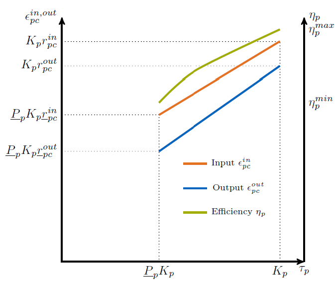
Many processes show a non-trivial part-load behavior. In particular, often a nonlinear reaction of the efficiency on the operational state is given. Although urbs itself is a linear program this can with some caveats be captured in many cases. The reason for this is, that the efficiency of a process is itself not given as a parameter, but is merely the ratio between input and output multipliers. It is thus possible to use purely linear functions to get a nonlinear behavior of the efficiency of the form:

\[\eta=\frac{a+b\tau_{pt}}{c+d\tau_{pt}},\]

where a,b,c and d are some constants. Specifically, the input and output ratios can be set to vary linearly between their respective values at full load \(r^{\text{in,out}}_{pc}\) and their values at the minimal allowed operational state \(\underline{P}_{p}\kappa_p\), which are given by \(\underline{r}^{\text{in,out}}_{pc}\). This is achieved with the following equations and exemplified with the following graphic:

\[\begin{split}&\forall p\in P^{\text{part load}},~c\in C,~t\in T_m:\\\\ &\epsilon^{\text{in,out}}_{pct}=\Delta t\cdot\left( \frac{\underline{r}^{\text{in,out}}_{pc}-r^{\text{in,out}}_{pc}} {1-\underline{P}_p}\cdot \underline{P}_p\cdot \kappa_p+ \frac{r^{\text{in,out}}_{pc}- \underline{P}_p\underline{r}^{\text{in,out}}_{pc}} {1-\underline{P}_p}\cdot \tau_{pt}\right).\end{split}\]

A few restrictions have to be kept in mind when using this feature:

• \(\underline{P}_p\) has to be set larger than 0 otherwise the feature will work but not have any effect.
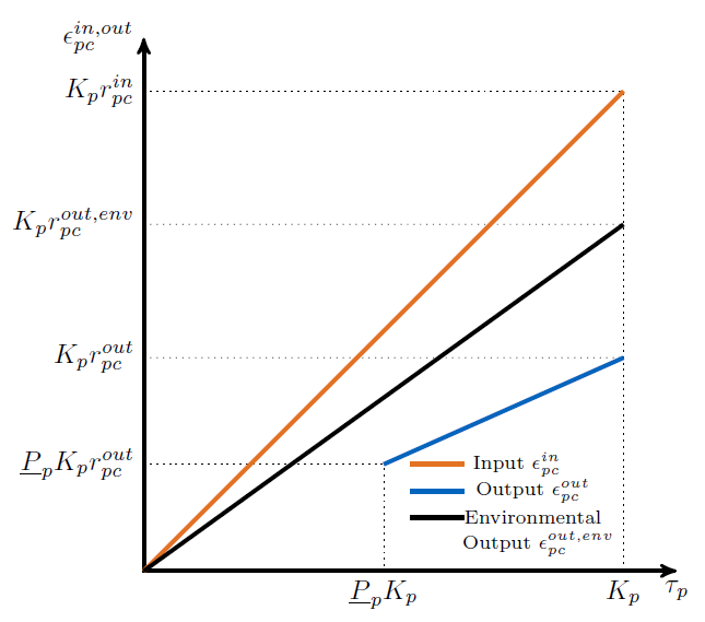
• Environmental output commodities have to mimic the behavior of the inputs by which they are generated. Otherwise the emissions per unit of input would change together with the efficiency, which is typically not the desired behavior.

On/off Behavior

Some processes are characterised by a minimum or part-load behavior but still retain the practical necessity of being turned on and off if this is optimal. This feature transforms urbs from a linear problem to a quadratic integer problem, or piecewise linear. The following graphic illustrates a process with the on/off feature and constant efficiency:

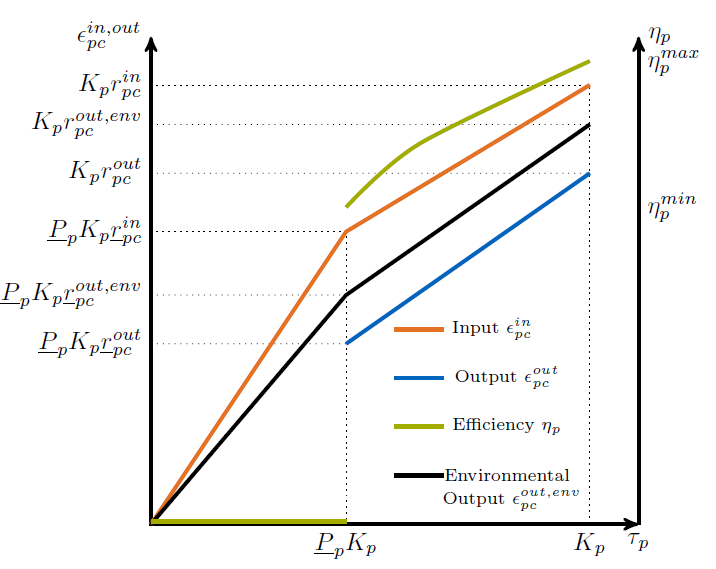
The following graphic illustrates a process with the on/off feature and part load behavior:

Coupling the throughput ant the on/off marker: The following equation introduces a coupling between \(\omicron_{pt}\), the boolean on/off marker of a process and its throughput \(\tau_{pt}\), so that \(\omicron_{pt}\) assumes the value 1 when the process has a non-zero output and 0 otherwise.

\[\begin{split}&\forall p\in P^{\text{on/off}},~t\in T_m:\\\\ &\underline{P}_p\cdot \kappa_p\cdot \omicron_{pt}\leq \tau_{pt}\leq \kappa_p\cdot \omicron_{pt}+ \underline{P}_p\cdot \kappa_p\cdot (1 - \omicron_{pt})\end{split}\]

Input: The following equation describes the alteration of the input equation of a process with on/off and part-load behaviors due to the necessity of having a continuous, linear function defined on two intervals. The first interval represents the starting input of a process, while the second one represents the consumed input while also producing.

\[\begin{split}&\forall p\in P^{\text{on/off with part load}},~c\in C,~t\in T_m:\\\\ &\epsilon^{in}_{pct}= \tau_{pt}\cdot r^{\text{in}}_{pc}\cdot (1-\omicron_{pt})+ \Delta t\cdot\left( \frac{\underline{r}^{\text{in}}_{pc}-r^{\text{in}}_{pc}} {1-\underline{P}_p}\cdot \underline{P}_p\cdot \kappa_p+ \frac{r^{\text{in}}_{pc}- \underline{P}_p\underline{r}^{\text{in}}_{pc}} {1-\underline{P}_p}\cdot \tau_{pt}\right)\cdot \omicron_{pt}.\end{split}\]

In order to ensure the continuity property of the function, the input ratio used for the starting interval has to be one corresponding to the minimum partial load, using \(\underline{r}^{\text{in}}_{pc}\). This is a realistic value, since processes normally use, percentagewise, more fuel in relationship to the throughput when starting than at higher throughput values.

Output differentiation: The following equations differentiate whether an output commodity needs to be produced when a process is starting (e.g. environmental commodities) or not (e.g. electricity):

\[\begin{split}&\forall p\in P^{\text{on/off}},~c\in C^{\text{environmental}},~t\in T_m:\\\\ &\epsilon^{out}_{pct}= \tau_{pt}\cdot r^{\text{out}}_{pc}\\ &\forall p\in P^{\text{on/off}},~c\in C^{\text{non-environmental}},~t\in T_m:\\\\ &\epsilon^{out}_{pct}= \tau_pt\cdot r^{\text{out}}_{pc}\cdot \omicron_{pt}.\end{split}\]

If the process also shows part-load behavior, the previous two equations change to a similarly adapted version of the part-load output equation:

\[\begin{split}&\forall p\in P^{\text{on/off with part load}},~c\in C^{\text{environmental}},~t\in T_m:\\\\ &\epsilon^{out}_{pct}= \tau_pt\cdot r^{\text{out}}_{pc}\cdot (1-\omicron_{pt})+ \Delta t\cdot\left( \frac{\underline{r}^{\text{out}}_{pc}-r^{\text{out}}_{pc}} {1-\underline{P}_p}\cdot \underline{P}_p\cdot \kappa_p+ \frac{r^{\text{out}}_{pc}- \underline{P}_p\underline{r}^{\text{out}}_{pc}} {1-\underline{P}_p}\cdot \tau_{pt}\right)\cdot \omicron_{pt}\\\\ &\forall p\in P^{\text{on/off}},~c\in C^{\text{non-environmental}},~t\in T_m:\\\\ &\epsilon^{\text{out}}_{pct}=\Delta t\cdot\left( \frac{\underline{r}^{\text{out}}_{pc}-r^{\text{out}}_{pc}} {1-\underline{P}_p}\cdot \underline{P}_p\cdot \kappa_p+ \frac{r^{\text{out}}_{pc}- \underline{P}_p\underline{r}^{\text{out}}_{pc}} {1-\underline{P}_p}\cdot \tau_{pt}\right)\cdot \omicron_{pt}.\end{split}\]

Here, it is important to notice that the output of the environmental commodities becomes a continuous, piecewise linear function defined on two intervals. In order to ensure the continuity property of the function, the output ratio used for the starting interval has to be the partial one, \(\underline{r}^{\text{in}}_{pc}\). This is a realistic value, since processes normaly produce, percentagewise, more CO2 and/or other environmental commodities in relationship to the throughput when starting then at higher throughput values.

Output ramping-up limit: While ramping up a process which can be turned on and off with a defined ramping up gradient, the following unrealistic situation might occur: Due to the fact that in the minimum working point the process on/off marker \(\omicron_{pt}\) can be both 0 and 1, the output of a process might have unrealistic jumps after the starting process is completed. There are 3 possible cases, each solved with its own output ramping equation, as follows:

Case I: When

\[\begin{split}&\underline{P}_p\geq \overline{PG}_p^{\text{up}}\\ &\underline{P}_p\ \text{is a multiple of} \overline{PG}_p^\text{up}.\end{split}\]

Here, in order to ensure that the process behaves realistically, it is needed to ensure that the process starts producing in the minimum working point, \(\underline{P}_p\kappa_p\ r^{\text{out}}_{pc}\), and not at a higher value. This is done by the following equation:

\[\begin{split}&\forall p\in P^{\text{on/off, case I}},~c\in C,~t\in T_m:\\\\ &\epsilon^{out}_{pct}-\epsilon^{out}_{pc(t-1)}\leq \Delta t\underline{P}_p\kappa_{p} r^{\text{out}}_{pc}.\end{split}\]

If the process shows a part load behavior, the equation changes to:

\[\begin{split}&\forall p\in P^{\text{on/off with part load, case I}},~c\in C,~t\in T_m:\\\\ &\epsilon^{out}_{pct}-\epsilon^{out}_{pc(t-1)}\leq \Delta t\underline{P}_p\kappa_{p}\underline{r}^{\text{out}}_{pc}.\end{split}\]

If the process has a time variable efficiency, the equation changes to:

\[\begin{split}&\forall p\in P^{\text{on/off with TimeVarEff, case I}},~c\in C,~t\in T_m:\\\\ &\epsilon^{out}_{pct}-\epsilon^{out}_{pc(t-1)}\leq \Delta t\underline{P}_p\kappa_{p} r^{\text{out}}_{pc} f^{\text{out}}_{pt}.\end{split}\]

If the process has both a part load behavior and a time variable efficiency, the equation changes to:

\[\begin{split}&\forall p\in P^{\text{on/off with TimeVarEff, case I}},~c\in C,~t\in T_m:\\\\ &\epsilon^{out}_{pct}-\epsilon^{out}_{pc(t-1)}\leq \Delta t\underline{P}_p\kappa_{p}\underline{r}^{\text{out}}_{pc} f^{\text{out}}_{pt}.\end{split}\]

Case II: When

\[\begin{split}&\underline{P}_{p}>\overline{PG}_p^\text{up}\\ &\underline{P}_p\ \text{is not a multiple of} \overline{PG}_p^\text{up}.\end{split}\]

Here, in order to ensure that the process behaves realistically, it is needed to ensure that the process starts somewhere in the interval between the minimum working point \(\underline{P}_p\kappa_p\) and the point of the first multiple of \(\overline{PG}_p^\text{up}\) greater than \(\underline{P}_p\kappa_p\), which is \((⌊\frac{\underline{P}_p}{\overline{PG}_p^\text{up}}⌋ +1)\cdot \overline{PG}_p\), where ⌊ ⌋ is the rounded down number. This is done by the following equation:

\[\begin{split}&\forall p\in P^{\text{on/off, case II}},~c\in C,~t\in T_m:\\\\ &\epsilon^{out}_{pct}-\epsilon^{out}_{pc(t-1)}\leq \Delta t (⌊\frac{\underline{P}_p}{\overline{PG}_p^\text{up}}⌋+1) \overline{PG}_p\kappa_{p} r^{\text{out}}_{pc}.\end{split}\]

If the process shows a part load behavior, the equation changes to:

\[\begin{split}&\forall p\in P^{\text{on/off, case II}},~c\in C,~t\in T_m:\\\\ &\epsilon^{out}_{pct}-\epsilon^{out}_{pc(t-1)}\leq \Delta t (⌊\frac{\underline{P}_p}{\overline{PG}_p^\text{up}}⌋ +1) \overline{PG}_p\kappa_{p}\underline{r}^{\text{out}}_{pc}.\end{split}\]

If the process has a time variable efficiency, the equation changes to:

\[\begin{split}&\forall p\in P^{\text{on/off with TimeVarEff, case II}},~c\in C,~t\in T_m:\\\\ &\epsilon^{out}_{pct}-\epsilon^{out}_{pc(t-1)}\leq \Delta t (⌊\frac{\underline{P}_p}{\overline{PG}_p^\text{up}}⌋ +1) \overline{PG}_p\kappa_{p} r^{\text{out}}_{pc} f^{\text{out}}_{pt}.\end{split}\]

If the process has both a part load behavior and a time variable efficiency, the equation changes to:

\[\begin{split}&\forall p\in P^{\text{on/off with part load and TimeVarEff, case II}},~c\in C,~t\in T_m:\\\\ &\epsilon^{out}_{pct}-\epsilon^{out}_{pc(t-1)}\leq \Delta t (⌊\frac{\underline{P}_p}{\overline{PG}_p^\text{up}}⌋ +1) \overline{PG}_p\kappa_{p}\underline{r}^{\text{out}}_{pc} f^{\text{out}}_{pt}.\end{split}\]

Case III: When

\[\underline{P}_{p}<\overline{PG}_p^\text{up}.\]

Here, in order to ensure that the process behaves realistically, it is needed to ensure that the process starts somewhere in the interval between the minimum working point \(\underline{P}_p\kappa_p\) and the first ramping up point greater than 0, \(\overline{PG}_p^\text{up}\kappa_p\). This is done by the following equation:

\[\begin{split}&\forall p\in P^{\text{on/off, case III}},~c\in C,~t\in T_m:\\\\ &\epsilon^{out}_{pct}-\epsilon^{out}_{pc(t-1)}\leq \Delta t\overline{PG}_p^\text{up}\kappa_{p} r^{\text{out}}_{pc}.\end{split}\]

If the process shows a part load behavior, the equation changes to:

\[\begin{split}&\forall p\in P^{\text{on/off, case III}},~c\in C,~t\in T_m:\\\\ &\epsilon^{out}_{pct}-\epsilon^{out}_{pc(t-1)}\leq \Delta t\overline{PG}_p^\text{up}\kappa_{p}\underline{r}^{\text{out}}_{pc}.\end{split}\]

If the process has a time variable efficiency, the equation changes to:

\[\begin{split}&\forall p\in P^{\text{on/off with TimeVarEff, case III}},~c\in C,~t\in T_m:\\\\ &\epsilon^{out}_{pct}-\epsilon^{out}_{pc(t-1)}\leq \Delta t\overline{PG}_p^\text{up}\kappa_{p} r^{\text{out}}_{pc}\ f^{\text{out}}_{pt}.\end{split}\]

If the process has both a part load behavior and a time variable efficiency, the equation changes to:

\[\begin{split}&\forall p\in P^{\text{on/off with part load and TimeVarEff, case III}},~c\in C,~t\in T_m:\\\\ &\epsilon^{out}_{pct}-\epsilon^{out}_{pc(t-1)}\leq \Delta t\overline{PG}_p^\text{up}\kappa_{p}\underline{r}^{\text{out}}_{pc} f^{\text{out}}_{pt}.\end{split}\]

Starting ramp-up: There are some processes which have a different ramping up gradient while starting than while producing. This is usually defined with the help of a so called starting time. The following equations transform the starting time into a starting ramp and implement the starting ramp only during start, either as the only ramping constraint when no ramp up gradient is defined or by replacing during start the rampiong up constraint which uses the ramping up gradient:

\[\begin{split}&\forall p\in P^{\text{on/off with start time}},~t\in T_m:\\\\ &SR_{p}= \frac{\underline{P}_p}{ST_{p}}\\ &\tau_{pt}-\tau_{p(t-1)}\leq \Delta t\overline{PG}_p^{\text{up}}\kappa_{p}\omicron_{p(t-1)}+ \Delta t\ SR_p \kappa_{p}(1-\omicron_{p(t-1)}).\end{split}\]

Start-up costs: For those processes which have a fix start-up cost, it is necessary to identify whether a process has completed its starting phase and begins to produce or not. The following equation does this by turning the boolean variable process start-up marker \(\sigma_{pt}\) to 1 when the process on/off marker switches from 0 to 1:

\[\begin{split}&\forall p\in P^{\text{on/off with start cost}},~t\in T_m:\\\\ &\sigma_{pt}\geq \omicron_{pt}-\omicron_{p(t-1)}.\end{split}\]

The following table shows the possible values of \(\sigma_{pt}\): .. table:: Table: Process Start-up Marker Values

\(\omicron_{pt}\)	\(\omicron_{p(t-1)}\)	\(\sigma_{pt}\)
0	0	0 or 1 (0 is optimal)
0	1	0
1	0	1
1	1	0

Costs

The cost function is ammended with one cost type, the start-up cost:

\[\zeta = \zeta_{\text{inv}} + \zeta_{\text{fix}} + \zeta_{\text{var}} + \zeta_{\text{fuel}} + \zeta_{\text{startup}} + \zeta_{\text{env}}.\]

Turning on a process requires sometime an additional fix cost besides the fuel used for the starting. As the variable costs, these costs occur when processes are used:

\[\begin{split}\zeta_{\text{startup}}=w \Delta t \sum_{t \in T_m\\ p \in P_{\text{on/off}}} {P}_p^\text{start}\sigma_{pt},\end{split}\]

where \({P}_p^\text{start}\) is the fix start-up cost and \(\sigma_{pt}\) is the process start-up marker. This cost type can also be merged into the same class of costs as the variable and fuel costs.