Process Constraints
Process Capacity Rule: The constraint process capacity rule defines the variable total process capacity \(\kappa_{vp}\). The variable total process capacity is defined by the constraint as the sum of the parameter process capacity installed \(K_{vp}\) and the variable new process capacity \(\hat{\kappa}_{vp}\). In mathematical notation this is expressed as:
In script urbs.py the constraint process capacity rule is defined and calculated by the following code fragment:
m.def_process_capacity = pyomo.Constraint(
    m.pro_tuples,
    rule=def_process_capacity_rule,
    doc='total process capacity = inst-cap + new capacity')
Process Input Rule: The constraint process input rule defines the variable process input commodity flow \(\epsilon_{vcpt}^\text{in}\). The variable process input commodity flow is defined by the constraint as the product of the variable process throughput \(\tau_{vpt}\) and the parameter process input ratio \(r_{pc}^\text{in}\). In mathematical notation this is expressed as:
In script urbs.py the constraint process input rule is defined and calculated by the following code fragment:
m.def_process_input = pyomo.Constraint(
    m.tm, m.pro_input_tuples - m.pro_partial_input_tuples,
    rule=def_process_input_rule,
    doc='process input = process throughput * input ratio')
Process Output Rule: The constraint process output rule defines the variable process output commodity flow \(\epsilon_{vcpt}^\text{out}\). The variable process output commodity flow is defined by the constraint as the product of the variable process throughput \(\tau_{vpt}\) and the parameter process output ratio \(r_{pc}^\text{out}\). In mathematical notation this is expressed as:
In script urbs.py the constraint process output rule is defined and calculated by the following code fragment:
m.def_process_output = pyomo.Constraint(
    m.tm, m.pro_output_tuples,
    rule=def_process_output_rule,
    doc='process output = process throughput * output ratio')
Intermittent Supply Rule: The constraint intermittent supply rule defines the variable process input commodity flow \(\epsilon_{vcpt}^\text{in}\) for processes \(p\) that use a supply intermittent commodity \(c \in C_\text{sup}\) as input. Therefore this constraint only applies if a commodity is an intermittent supply commodity \(c \in C_\text{sup}\). The variable process input commodity flow is defined by the constraint as the product of the variable total process capacity \(\kappa_{vp}\) and the parameter intermittent supply capacity factor \(s_{vct}\). In mathematical notation this is expressed as:
In script urbs.py the constraint intermittent supply rule is defined and calculated by the following code fragment:
m.def_intermittent_supply = pyomo.Constraint(
    m.tm, m.pro_input_tuples,
    rule=def_intermittent_supply_rule,
    doc='process output = process capacity * supim timeseries')
Process Throughput By Capacity Rule: The constraint process throughput by capacity rule limits the variable process throughput \(\tau_{vpt}\). This constraint prevents processes from exceeding their capacity. The constraint states that the variable process throughput must be less than or equal to the variable total process capacity \(\kappa_{vp}\). In mathematical notation this is expressed as:
In script urbs.py the constraint process throughput by capacity rule is defined and calculated by the following code fragment:
m.res_process_throughput_by_capacity = pyomo.Constraint(
    m.tm, m.pro_tuples,
    rule=res_process_throughput_by_capacity_rule,
    doc='process throughput <= total process capacity')
Process Throughput Gradient Rule: The constraint process throughput gradient rule limits the process power gradient \(\left| \tau_{vpt} - \tau_{vp(t-1)} \right|\). This constraint prevents processes from exceeding their maximal possible change in activity from one time step to the next. The constraint states that absolute power gradient must be less than or equal to the maximal power gradient \(\overline{PG}_{vp}\) parameter (scaled to capacity and by time step duration). In mathematical notation this is expressed as:
In script urbs.py the constraint process throughput gradient rule is defined and calculated by the following code fragment:
m.res_process_throughput_gradient = pyomo.Constraint(
    m.tm, m.pro_tuples,
    rule=res_process_throughput_gradient_rule,
    doc='process throughput gradient <= maximal gradient')
Process Capacity Limit Rule: The constraint process capacity limit rule limits the variable total process capacity \(\kappa_{vp}\). This constraint restricts a process \(p\) in a site \(v\) from having more total capacity than an upper bound and having less than a lower bound. The constraint states that the variable total process capacity \(\kappa_{vp}\) must be greater than or equal to the parameter process capacity lower bound \(\underline{K}_{vp}\) and less than or equal to the parameter process capacity upper bound \(\overline{K}_{vp}\). In mathematical notation this is expressed as:
In script urbs.py the constraint process capacity limit rule is defined and calculated by the following code fragment:
m.res_process_capacity = pyomo.Constraint(
    m.pro_tuples,
    rule=res_process_capacity_rule,
    doc='process.cap-lo <= total process capacity <= process.cap-up')
Sell Buy Symmetry Rule: The constraint sell buy symmetry rule defines the total process capacity \(\kappa_{vp}\) of a process \(p\) in a site \(v\) that uses either sell or buy commodities ( \(c \in C_\text{sell} \vee C_\text{buy}\)), therefore this constraint only applies to processes that use sell or buy commodities. The constraint states that the total process capacities \(\kappa_{vp}\) of processes that use complementary buy and sell commodities must be equal. Buy and sell commodities are complementary, when a commodity \(c\) is an output of a process where the buy commodity is an input, and at the same time the commodity \(c\) is an input commodity of a process where the sell commodity is an output.
In script urbs.py the constraint sell buy symmetry rule is defined and calculated by the following code fragment:
m.res_sell_buy_symmetry = pyomo.Constraint(
    m.pro_input_tuples,
    rule=res_sell_buy_symmetry_rule,
    doc='total power connection capacity must be symmetric in both directions')
Partial & Startup Process Constraints
It is important to understand that this partial load formulation can only work if its accompanied by a sensible value for both the minimum partial load fraction \(\underline{P}_{vp}\) and the startup cost \(k_{vp}^\text{startup}\). Otherwise, the optimal solution yields identical operation and performance like a regular, fully proportional process with constant/flat input ratios.
Throughput by Online Capacity Min Rule
The new variable online capacity forces the process throughput to always stay above its value times the minium partial load fraction. But note that there is no constraint that stops \(\omega_{vpt}\) from assuming arbitrarily small values. This is only softly prohibited by the startup cost term, which acts as kind of a soft friction term that punishes too dynamic of an operation strategy.
And here as code:
m.res_throughput_by_online_capacity_min = pyomo.Constraint(
    m.tm, m.pro_partial_tuples,
    rule=res_throughput_by_online_capacity_min_rule,
    doc='cap_online * min-fraction <= tau_pro')
Throughput by Online Capacity Max Rule
On the other side, the online capacity is an upper cap on the process throughput.
And the code:
m.res_throughput_by_online_capacity_max = pyomo.Constraint(
    m.tm, m.pro_partial_tuples,
    rule=res_throughput_by_online_capacity_max_rule,
    doc='tau_pro <= cap_online')
Partial Process Input Rule: In energy system modelling, the simplest way to represent an energy conversion process is to assume a linear input-output relationship with a flat efficiency parameter \(\eta\):
Which means there is only one efficiency \(\eta\) during the whole process, i.e. it remains constant during the electricity production. But in fact, most of the powerplants do not operate at a certain efficiency and the operation load varies along time. Therefore the regular single efficiency \(\eta\) will be replaced by a set of input ratios (\(r^\text{in}\)) and output ratios (\(r^\text{out}\)) in urbs. And both ratios relate to the process activity \(\tau\):
In order to simplify the mathematical calculation, the output ratios are set to 1 so that the process output (\(\epsilon_{pct}^\text{out}\)) is equal to the process throughput (\(\tau\)). Then, the process efficiency \(\eta\) can be represented as follows:
Assume now a process, it has a lower input ratio \(\underline{r}_{pc}^\text{in}\), a upper input ratio \(r_{pc}^\text{in}\), the process minimum part load fraction \(\underline{P}_{vp}\) and the corresponding start-up costs. The \(\tau\) will be bounded by \(\underline{P}_{vp}\) and the online capacity \(\omega_{vpt}\), which means the throughput can only vary between \(\underline{P}_{vp} \cdot \omega_{vpt}\) and \(\omega_{vpt}\). When all the start-up costs are equal to zero, the relation between the process input and the process throughout is nothing else but a straight line across the original point, which exists almost only theoretically. Practically, every powerplant has a start-up cost, which has a big influence on the effeiciency of the process.
To research the influence of the start-up costs, a continouous start-up variable \(\chi_{pt} \in [0, \kappa_p]\) is introduced and defines as follows:
Where the \(\omega_{pt}\) is also a new introduced variable, represents the start-up capacity (or the idle consumption). With these two variables, the urbs can detect the energy consumption of a process at the starting point and put a start-up costs on it to obtain the variable costs.
As it is not immediately clear what this expression accomplishes, here is visual example. It plots the value off the expression \(\tau_{vpt}/\epsilon_{vpct}^\text{in}\) for a process with \(\underline{P}_{vp} = 0.35\), \(\underline{r}_{pc}^\text{in} = 3.33\) and \(r_{pc}^\text{in} = 2.5\) and a hypothetical capacity of \(1 MW\). When operating at its maximum, it yields an input efficiecny of \(40 \%\), whereas in partial load this drops to \(30 \%\).
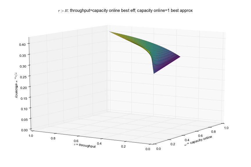
More discussion and a visualisation of the reverse case (partial load more efficient than full load operation) is shown in a dedicated IPython notebook.
m.def_partial_process_input = pyomo.Constraint(
    m.tm, m.pro_partial_input_tuples,
    rule=def_partial_process_input_rule,
    doc='e_pro_in = cap_online * min_fraction * (r - R) / (1 - min_fraction)'
                    '+ tau_pro * (R - min_fraction * r) / (1 - min_fraction)')
Online Capacity By Process Capacity Rule limits the value of the online capacity \(\omega_{vpt}\) by the total installed process capacity \(\kappa_{vp}\):
m.res_cap_online_by_cap_pro = pyomo.Constraint(
    m.tm, m.pro_partial_tuples,
    rule=res_cap_online_by_cap_pro_rule,
    doc='online capacity <= process capacity')
Startup Capacity Rule determines the value of the startup capacity indicator variable \(\phi_{vpt}\), by limiting its value to at least the positive difference of subsequent online capacity states \(\omega_{vpt}\) and \(\omega_{vp(t-1)}\). In other words: whenever the onlince capacity increases, startup capacity \(\phi_{vpt}\) assumes a non-zero value.
Code declaration and definition:
m.def_startup_capacity = pyomo.Constraint(
    m.tm, m.pro_partial_tuples,
    rule=def_startup_capacity_rule,
    doc='startup_capacity[t] >= cap_online[t] - cap_online[t-1]')